Getting Started with Stan
Bayesian Workflow
In general the Bayesian workflow consists of steps:
- Consider the social process that generates your data. The goal of your statistical model should be to model the data generating process, so think hard about this. Exploratory analysis goes a long way towards helping you to understand this process.
- Program your statistical model and sample from it.
- Evaluate your model’s reliability. Check for Markov chain convergence to make sure that your model has produced reliable estimates.
- Evaluate your model’s performance. How well does your model approximate the data generating process? This involves using posterior predictive checks.
- Summarize your model’s results in tabular and graphical form.
What is Stan?
In this tutorial, we’ll walk through the basics of the Stan programming language. You can interface with Stan through almost any data analysis language (R, Python, shell, MATLAB, Julia, or Stata), but I will be interfacing with it in R.
Stan is an open-source software that uses No-U-Turn Hamiltonian Monte Carlo for Bayesian inference and is named after one of the creators of the Monte Carlo method, Stanislaw Ulam.
Interfacing with Stan through R
In order to use Stan, you need to install it. The process is fairly straightforward, but the steps vary slightly depending on your operation system. See this help page for the details of installation.
Assuming you have a C++ compiler installed (follow the steps linked above), RStan can be installed by typing:
install.packages("rstan",
                 repos = "https://cloud.r-project.org/",
                 dependencies = TRUE)
After installation, let’s load the RStan library.
library(rstan)## Loading required package: StanHeaders## Loading required package: ggplot2## rstan (Version 2.21.3, GitRev: 2e1f913d3ca3)## For execution on a local, multicore CPU with excess RAM we recommend calling
## options(mc.cores = parallel::detectCores()).
## To avoid recompilation of unchanged Stan programs, we recommend calling
## rstan_options(auto_write = TRUE)Stan Syntax
Stan requires the coding of your model in different blocks and in a specific order. In order, these blocks are data, transformed data, parameters, transformed parameters, model, and generated quantities. Let’s suppose that we wanted to estimate the following equation with Stan:
\[ \begin{aligned} y &\sim \text{Normal}(\mu, \sigma) \\ \mu &= \alpha + \beta x \\ \alpha &\sim \text{Normal}(0, 10) \\ \beta &\sim \text{Normal}(0, 10) \\ \sigma &\sim \text{Uniform}(0, 100) \\ \end{aligned} \]
A complete Stan program for this model looks like the following:
data { // This is the data block
  int N; // Specify Sample Size
  real y[N]; // A variable named y with length n
  real x[N]; // A variable named x with length n
}

transformed data {
  // this is where you could specify variable transformations
}

parameters { // Block for parameters to be estimated
  real a; // A parameter named a
  real b; // A parameter named b
  real sigma; // A parameter named sigma
}

transformed parameters {
  // Here you could specify transformations of your parameters
}

model {
  vector[N] mu; // create the linear predictor mu

  // Write the linear model
  for (i in 1:N) {
    mu[i] = a + b * x[i];
  }

  // Write out priors
  a ~ normal(0, 10);
  b ~ normal(0, 10);
  sigma ~ uniform(0, 100);

  // Write out the likelihood function
  for (i in 1:N) {
  y[i] ~ normal(mu[i], sigma);
  }
}

generated quantities {
  // Here you can calculate things like log-likelihood, replication data, etc.
}
After programming the model, you run the code which will tell R to compile it into a model. From there we are ready to sample from the model. Note that Stan is case sensitive and each line must terminate with a semi-colon “;”.
Example!
Exploratory Analysis
Let’s get going with an example using mpg data.
mpg.data <- mpg

library(tidyverse)
## ── Attaching packages ─────────────────────────────────────── tidyverse 1.3.1 ──## ✓ tibble 3.1.6 ✓ dplyr 1.0.7
## ✓ tidyr 1.1.4 ✓ stringr 1.4.0
## ✓ readr 2.1.1 ✓ forcats 0.5.1
## ✓ purrr 0.3.4## ── Conflicts ────────────────────────────────────────── tidyverse_conflicts() ──
## x tidyr::extract() masks rstan::extract()
## x dplyr::filter() masks stats::filter()
## x dplyr::lag() masks stats::lag()glimpse(mpg)## Rows: 234
## Columns: 11
## $ manufacturer <chr> "audi", "audi", "audi", "audi", "audi", "audi", "audi", "…
## $ model <chr> "a4", "a4", "a4", "a4", "a4", "a4", "a4", "a4 quattro", "…
## $ displ <dbl> 1.8, 1.8, 2.0, 2.0, 2.8, 2.8, 3.1, 1.8, 1.8, 2.0, 2.0, 2.…
## $ year <int> 1999, 1999, 2008, 2008, 1999, 1999, 2008, 1999, 1999, 200…
## $ cyl <int> 4, 4, 4, 4, 6, 6, 6, 4, 4, 4, 4, 6, 6, 6, 6, 6, 6, 8, 8, …
## $ trans <chr> "auto(l5)", "manual(m5)", "manual(m6)", "auto(av)", "auto…
## $ drv <chr> "f", "f", "f", "f", "f", "f", "f", "4", "4", "4", "4", "4…
## $ cty <int> 18, 21, 20, 21, 16, 18, 18, 18, 16, 20, 19, 15, 17, 17, 1…
## $ hwy <int> 29, 29, 31, 30, 26, 26, 27, 26, 25, 28, 27, 25, 25, 25, 2…
## $ fl <chr> "p", "p", "p", "p", "p", "p", "p", "p", "p", "p", "p", "p…
## $ class <chr> "compact", "compact", "compact", "compact", "compact", "c…This data set contains data on the make and model over different cars along with their engine type, transmission type, and mpg. Let’s do some visualizations to get a better understanding of our data.
ggplot(data = mpg.data,
       aes(x = cyl, y = cty)) +
  geom_point() +
  geom_smooth(method = "lm") +
  theme_bw(base_size = 14) +
  labs(x = "Engine Size",
       y = "City MPG",
       title = "Engine Size vs. City MPG")
## `geom_smooth()` using formula 'y ~ x'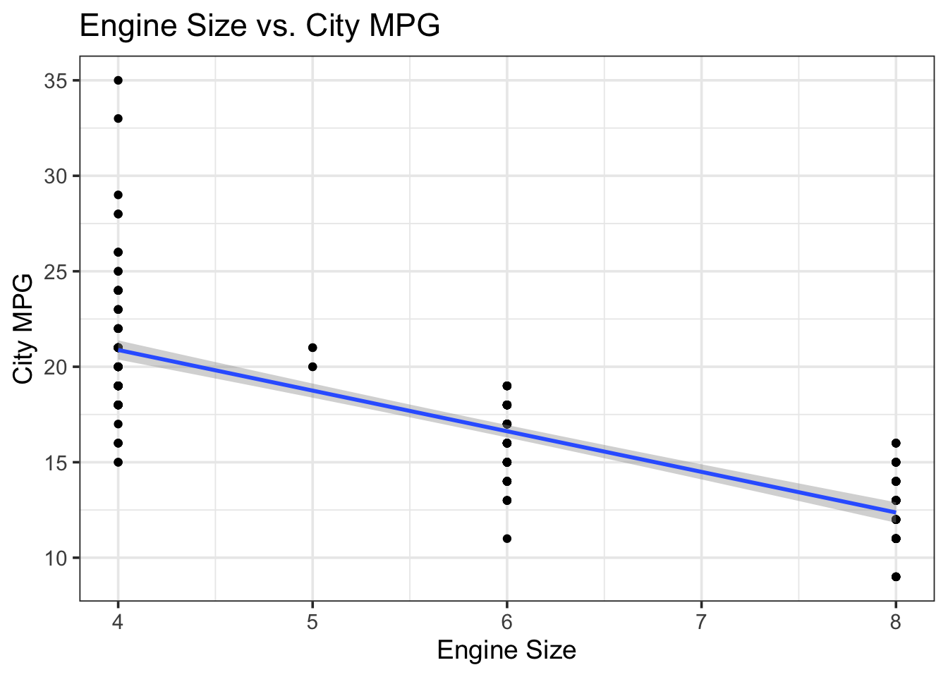
As expected, there is a negative relationship between engine size and city MPG. Let’s build a simple linear model to see if engine type affects mpg. In mathematical notation, this model would look like:
\[ \begin{aligned} \text{mpg}_i &\sim \text{Normal}(\mu_i, \sigma) \\ \mu_i &= \alpha + \beta \cdot \text{Engine}_i \\ \alpha &\sim \text{Normal}(0, 100) \\ \beta &\sim \text{Normal}(0, 100) \\ \sigma &\sim \text{Uniform}(0, 100) \\ \end{aligned} \]
Prior Simulations
Notice that I am specifying pretty uninformative priors. To see just how uninformative, let’s do some simulations. Centering continuous variables can also help to interpret priors.
# use rnorm to draw from a normal distribution
sim.data <- rnorm(n = 10000, mean = 0, sd = 100)

# convert the sim.data to a data frame (it's stored as a vector right now)
sim.data <- as.data.frame(sim.data)

# now let's plot it
ggplot() +
  geom_density(data = sim.data, aes(x = sim.data)) +
  # it's a good idea to label your axes to help you understand the units
  xlab("Effect Range of Engine Type on MPG")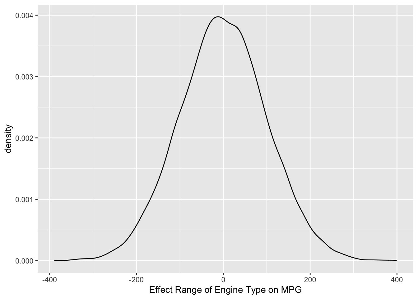
So, we are telling the model that the average effect of engine type on MPG will be zero, but can range between a decrease of 200 and an increase of 200 MPG with reasonably high probability. Thus, this is a pretty flat prior. Cars with bigger engines will probably get lower MPG, but they probably don’t get 200 MPG lower! This is a good time to point out that uninformative priors are rarely ever a good idea since we almost always know something about the effects we are interested in before we estimate them.
Finally, let’s examine the prior for \(\sigma\).
# draw from a uniform distribution
sim.data <- runif(n = 10000, min = 0, max = 100)

# convert to a data from
sim.data <- as.data.frame(sim.data)

# now plot
ggplot() +
  geom_density(data = sim.data, aes(x = sim.data)) +
  xlab("Model Variance")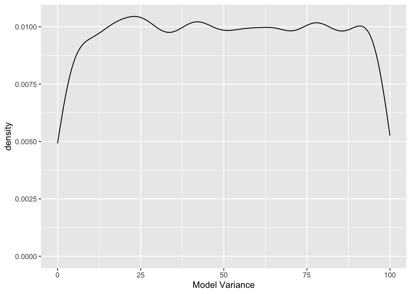
Model Programming
Now that we know what we are telling the model a priori, let’s program the model. We’ll program it in three different ways to showcase the various options available in Stan. Also, when using Stan in R Markdown, you’ll want to assign each Stan program an output name. You can do this by specifying the output.var = in the code chunk options.
Vectorized Syntax
data {
  int n; // number of observations (rows of data)
  vector[n] mpg; // variable called mpg as a vector of length n
  vector[n] engine; // variable called weight as a vector of length n
}

parameters {
  real alpha; // this will be our intercept
  real beta; // this will be our slope
  real sigma; // this will be our variance parameter
}

model {
  // create the linear predictor
  vector[n] mu;

  // write the linear combination
  mu = alpha + beta * engine;

  // priors
  alpha ~ normal(0, 100);
  beta ~ normal(0, 100);
  sigma ~ uniform(0, 100);

  // write the likelihood
  mpg ~ normal(mu, sigma);
}

generated quantities {
  vector[n] log_lik; // calculate log-likelihood
  vector[n] y_rep; // replications from posterior predictive distribution

  for (i in 1:n) {
    // generate mpg predicted value
    real mpg_hat = alpha + beta * engine[i];

    // calculate log-likelihood
    log_lik[i] = normal_lpdf(mpg[i] | mpg_hat, sigma);
    // normal_lpdf is the log of the normal probability densift function

    // generate replication values
    y_rep[i] = normal_rng(mpg_hat, sigma);
    // normal_rng generates random numbers from a normal distribution
  }
}
Unvectorized Syntax
As an alternative to the vectorized syntax above, we could also program the model using unvectorized syntax. This is necessary with some types of models that don’t support vectorized notation. In general, the vectorized syntax is much more efficient. We’ll called this the unvectorized model output.var = "unvec.model". Notice that with the unvectorized syntax, we tell the model what type of data our variables are. mpg and engine are real numbers.
data {
  int n; // number of observations (rows of data)
  real mpg[n]; // variable called mpg as a vector of length n
  real engine[n]; // variable called weight as a vector of length n
}

parameters {
  real alpha; // this will be our intercept
  real beta; // this will be our slope
  real sigma; // this will be our variance parameter
}

model {
  // create the linear predictor
  vector[n] mu;

  // write the linear combination
  for (i in 1:n) {
    mu[i] = alpha + beta * engine[i];
  }

  // priors
  alpha ~ normal(0, 100);
  beta ~ normal(0, 100);
  sigma ~ uniform(0, 100);

  // write the likelihood
  for (i in 1:n) {
    mpg[i] ~ normal(mu[i], sigma);
  }
}

generated quantities {
  vector[n] log_lik; // calculate log-likelihood
  vector[n] y_rep; // replications from posterior predictive distribution

  for (i in 1:n) {
    // generate mpg predicted value
    real mpg_hat = alpha + beta * engine[i];

    // calculate log-likelihood
    log_lik[i] = normal_lpdf(mpg[i] | mpg_hat, sigma);
    // normal_lpdf is the log of the normal probability densift function

    // generate replication values
    y_rep[i] = normal_rng(mpg_hat, sigma);
    // normal_rng generates random numbers from a normal distribution
  }
}
Target+ Syntax
Finally, Stan allows users to directly specify the log-posterior using target+ syntax. Using this syntax, y ~ normal(mu, sigma); becomes target += normal_lpdf(y | mu, sigma). This directly updates the target log density.
data {
  int n; // number of observations (rows of data)
  vector[n] mpg; // variable called mpg as a vector of length n
  vector[n] engine; // variable called weight as a vector of length n
}

parameters {
  real alpha; // this will be our intercept
  real beta; // this will be our slope
  real sigma; // this will be our variance parameter
}

model {
  // create the linear predictor
  vector[n] mu;

  // write the linear combination
  mu = alpha + beta * engine;

  target += normal_lpdf(alpha | 0, 100);
  target += normal_lpdf(beta | 0, 100);
  target += uniform_lpdf(sigma | 0, 100);
  target += normal_lpdf(mpg | mu, sigma);
}

generated quantities {
  vector[n] log_lik; // calculate log-likelihood
  vector[n] y_rep; // replications from posterior predictive distribution

  for (i in 1:n) {
    // generate mpg predicted value
    real mpg_hat = alpha + beta * engine[i];

    // calculate log-likelihood
    log_lik[i] = normal_lpdf(mpg[i] | mpg_hat, sigma);
    // normal_lpdf is the log of the normal probability densift function

    // generate replication values
    y_rep[i] = normal_rng(mpg_hat, sigma);
    // normal_rng generates random numbers from a normal distribution
  }
}
Now, let’s get into running some linear models.