Multilevel Modeling in Stan
There are a few different ways to model data that contains repeated observations for units over time, or that is nested within groups. First, we could simply pool all the data together and ignore the nested structure (pooling). Second, we could consider observations from each group as entirely independent from observations in other groups (no pooling). Finally, we could use information about the similarity of observations within groups to inform our individual estimates (partial pooling).
Import Data
library(pacman)
p_load(rstanarm, cmdstanr, tidyverse)

register_knitr_engine(override = FALSE) # This registers cmdstanr with knitr so that we can use
# it with R Markdown.

data(radon)
Pooling
Let’s start with the pooling estimates. As a point of reference, we’ll fit a frequentist model first.
Frequentist Fit
# fit model
pooling.fit <- lm(formula = log_radon ~ floor, data = radon)

# print results
library(broom)
library(broom.mixed)
tidy(pooling.fit, conf.int = TRUE)
## # A tibble: 2 × 7
## term estimate std.error statistic p.value conf.low conf.high
## <chr> <dbl> <dbl> <dbl> <dbl> <dbl> <dbl>
## 1 (Intercep… 1.36 0.0285 47.7 9.17e-251 1.31 1.42
## 2 floor -0.586 0.0700 -8.38 1.95e- 16 -0.724 -0.449# calculate fitted values
radon$pooling.fit <- fitted(pooling.fit)
# plot the model results
ggplot(data = radon, aes(x = as_factor(floor), y = log_radon, group = county)) +
geom_line(aes(y = pooling.fit), color = "black") +
geom_point(alpha = 0.3,
size = 3,
position = position_jitter(width = 0.1, height = 0.2)) +
facet_wrap(~ county) +
ggpubr::theme_pubr()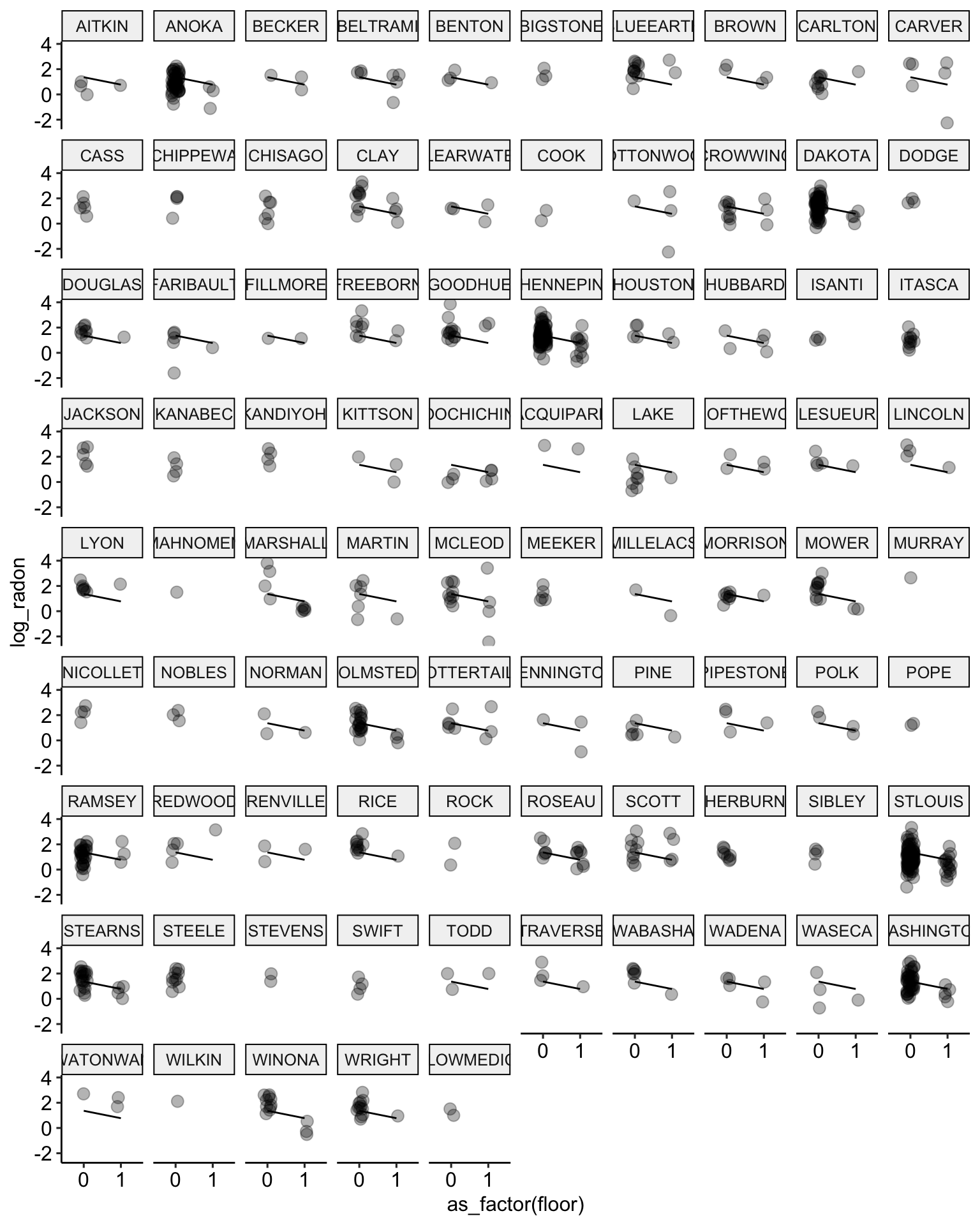
Bayesian Fit
Program the model in Stan.
data {
  int n; // number of observations
  vector[n] log_radon;
  vector[n] vfloor;
}

parameters {
  real alpha; // intercept parameter
  real beta; // slope parameter
  real sigma; // variance parameter
}

model {
  // conditional mean
  vector[n] mu;

  // linear combination
  mu = alpha + beta * vfloor;

  // priors
  alpha ~ normal(0, 100);
  beta ~ normal(0, 100);
  sigma ~ uniform(0, 100);

  // likelihood function
  log_radon ~ normal(mu, sigma);
}

generated quantities {
  vector[n] log_lik; // calculate log-likelihood
  vector[n] y_rep; // replications from posterior predictive distribution

  for (i in 1:n) {
    // generate mpg predicted value
    real log_radon_hat = alpha + beta * vfloor[i];

    // calculate log-likelihood
    log_lik[i] = normal_lpdf(log_radon[i] | log_radon_hat, sigma);
    // normal_lpdf is the log of the normal probability density function

    // generate replication values
    y_rep[i] = normal_rng(log_radon_hat, sigma);
    // normal_rng generates random numbers from a normal distribution
  }
}
Now we fit this model:
# prepare data for stan
library(tidybayes)
model.data <-
  radon %>%
  rename(vfloor = floor) %>%
  dplyr::select(log_radon, vfloor) %>%
  compose_data()

# fit stan model
stan.pooling.fit <- pooling.model$sample(data = model.data, refresh = 0)
## Running MCMC with 4 sequential chains...
##
## Chain 1 finished in 0.6 seconds.
## Chain 2 finished in 0.6 seconds.
## Chain 3 finished in 0.6 seconds.
## Chain 4 finished in 0.7 seconds.
##
## All 4 chains finished successfully.
## Mean chain execution time: 0.6 seconds.
## Total execution time: 3.0 seconds.library(rstan)
stan.pooling.fit <- read_stan_csv(stan.pooling.fit$output_files())
tidy(stan.pooling.fit)## # A tibble: 1,841 × 3
## term estimate std.error
## <chr> <dbl> <dbl>
## 1 alpha 1.36 0.0291
## 2 beta -0.588 0.0721
## 3 sigma 0.791 0.0188
## 4 log_lik[1] -0.691 0.0247
## 5 log_lik[2] -0.910 0.0281
## 6 log_lik[3] -0.741 0.0246
## 7 log_lik[4] -1.97 0.0688
## 8 log_lik[5] -0.718 0.0243
## 9 log_lik[6] -0.818 0.0260
## 10 log_lik[7] -1.32 0.0418
## # … with 1,831 more rowsstan.pooling.values <-
stan.pooling.fit %>% # use this model fit
spread_draws(alpha, beta, sigma) %>% # extract samples in tidy format
median_hdci() # calculate the median HDCI
# plot the model results for the median estimates
ggplot(data = radon, aes(x = floor, y = log_radon, group = county)) +
geom_abline(data = stan.pooling.values,
aes(intercept = alpha, slope = beta), color = "black") +
geom_point(alpha = 0.3,
size = 3,
position = position_jitter(width = 0.1, height = 0.2)) +
facet_wrap(~ county) +
ggpubr::theme_pubr()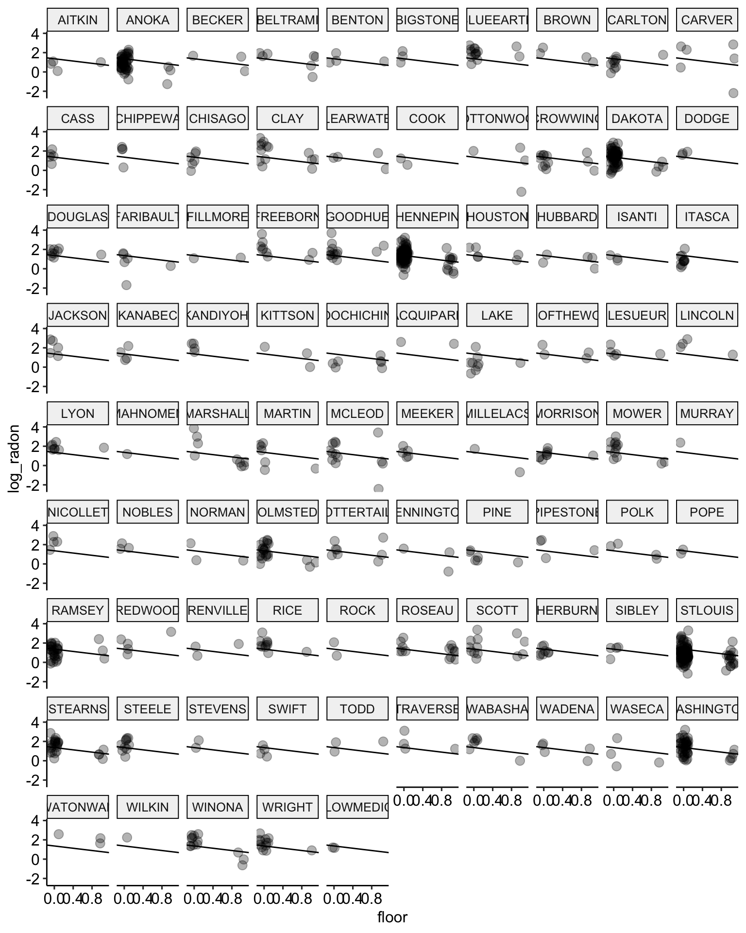
# plot the model results with posterior samples
stan.pooling.samples <-
  stan.pooling.fit %>% # use this model fit
  spread_draws(alpha, beta, sigma, n = 20) # extract 20 samples in tidy format

ggplot() +
  geom_abline(data = stan.pooling.samples,
            aes(intercept = alpha, slope = beta),
            color = "black",
            alpha = 0.3) +
  geom_point(data = radon,
             aes(x = floor, y = log_radon, group = county),
             alpha = 0.3,
             size = 3,
             position = position_jitter(width = 0.1, height = 0.2)) +
  facet_wrap(~ county) +
  ggpubr::theme_pubr()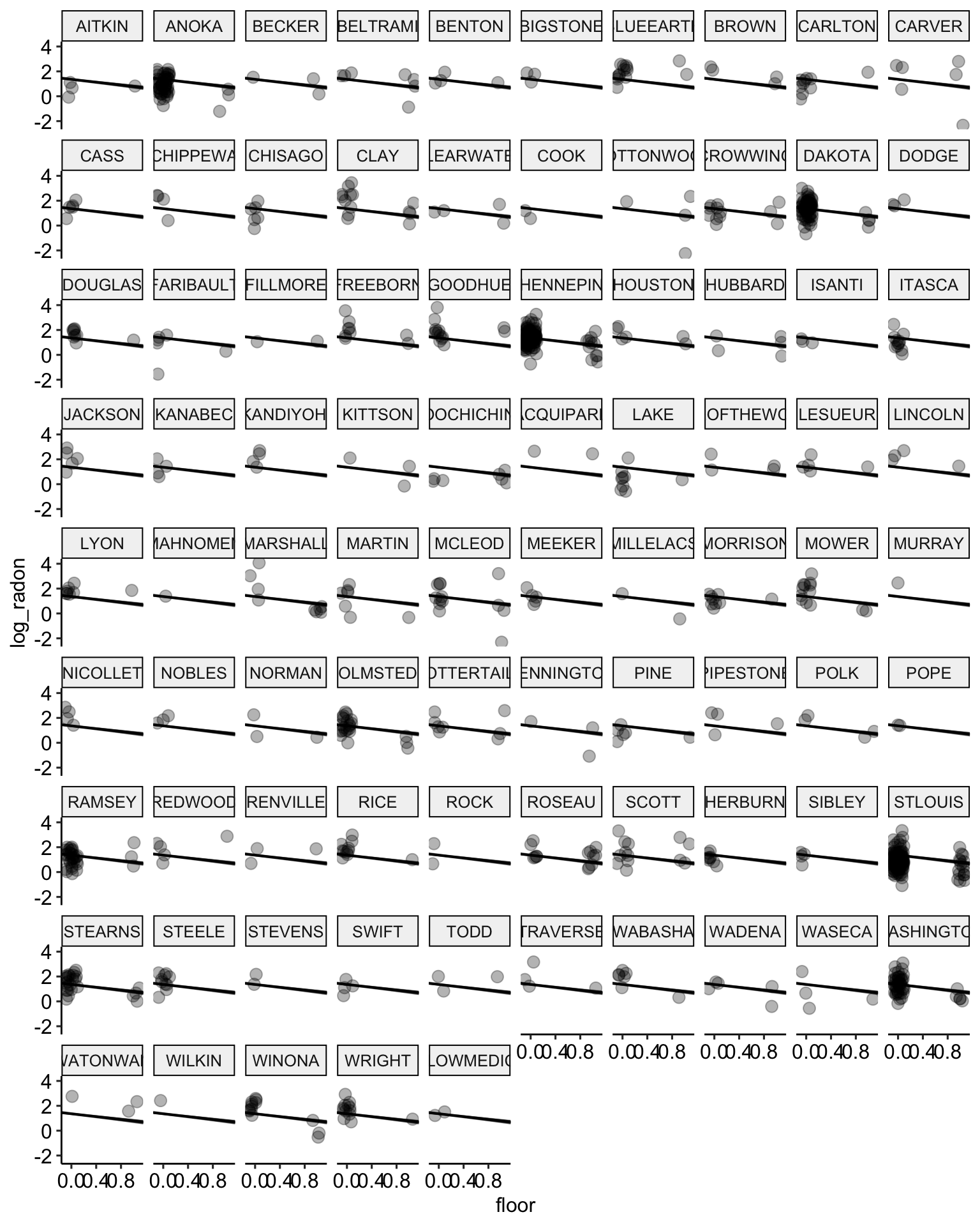
No Pooling
Now lets move to the no pooling estimates. These are sometimes referred to as “fixed-effects” by economists because you control for grouped data structures by including indicator variables to the grouping units. To give you a reference point, we’ll fit this model in a frequentist framework first.
Frequentist Fit
# fit the model without an intercept to include all 85 counties
no.pooling.fit <- lm(formula = log_radon ~ floor + as_factor(county) - 1,
                     data = radon)

# print results
tidy(no.pooling.fit, conf.int = TRUE)
## # A tibble: 86 × 7
## term estimate std.error statistic p.value conf.low conf.high
## <chr> <dbl> <dbl> <dbl> <dbl> <dbl> <dbl>
## 1 floor -0.689 0.0706 -9.76 2.22e-21 -0.828 -0.551
## 2 as_factor… 0.887 0.364 2.44 1.49e- 2 0.173 1.60
## 3 as_factor… 0.931 0.101 9.23 2.20e-19 0.733 1.13
## 4 as_factor… 1.55 0.422 3.67 2.57e- 4 0.721 2.38
## 5 as_factor… 1.59 0.278 5.72 1.50e- 8 1.04 2.13
## 6 as_factor… 1.45 0.364 4.00 6.92e- 5 0.741 2.17
## 7 as_factor… 1.54 0.419 3.66 2.64e- 4 0.713 2.36
## 8 as_factor… 2.02 0.194 10.4 5.87e-24 1.64 2.41
## 9 as_factor… 2.00 0.365 5.47 5.99e- 8 1.28 2.71
## 10 as_factor… 1.05 0.230 4.55 6.19e- 6 0.595 1.50
## # … with 76 more rows# calculate fitted values
radon$no.pooling.fit <- fitted(no.pooling.fit)
# plot the model results
ggplot(data = radon, aes(x = as_factor(floor), y = log_radon, group = county)) +
geom_line(aes(y = pooling.fit), color = "black") +
geom_line(aes(y = no.pooling.fit), color = "red") + # add no pooling estimates
geom_point(alpha = 0.3,
size = 3,
position = position_jitter(width = 0.1, height = 0.2)) +
facet_wrap(~ county) +
ggpubr::theme_pubr()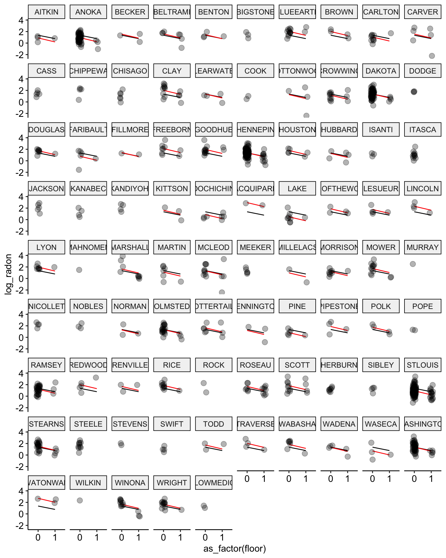
Bayesian Fit
Program the model in Stan.
data {
  int n; // number of observations
  int n_county; // number of counties
  vector[n] log_radon;
  vector[n] vfloor;
  int<lower = 0, upper = n_county> county[n];
}

parameters {
  vector[n_county] alpha; // vector of county intercepts
  real beta; // slope parameter
  real<lower = 0> sigma; // variance parameter
}

model {
  // conditional mean
  vector[n] mu;

  // linear combination
  mu = alpha[county] + beta * vfloor;

  // priors
  alpha ~ normal(0, 100);
  beta ~ normal(0, 100);
  sigma ~ uniform(0, 100);

  // likelihood function
  log_radon ~ normal(mu, sigma);
}

generated quantities {
  vector[n] log_lik; // calculate log-likelihood
  vector[n] y_rep; // replications from posterior predictive distribution

  for (i in 1:n) {
    // generate mpg predicted value
    real log_radon_hat = alpha[county[i]] + beta * vfloor[i];

    // calculate log-likelihood
    log_lik[i] = normal_lpdf(log_radon[i] | log_radon_hat, sigma);
    // normal_lpdf is the log of the normal probability density function

    // generate replication values
    y_rep[i] = normal_rng(log_radon_hat, sigma);
    // normal_rng generates random numbers from a normal distribution
  }
}
Now we fit this model:
# prepare data for stan
model.data <-
  radon %>%
  rename(vfloor = floor) %>%
  dplyr::select(log_radon, vfloor, county) %>%
  compose_data()

# fit stan model
stan.no.pooling.fit <- no.pooling.model$sample(data = model.data, refresh = 0)
## Running MCMC with 4 sequential chains...
##
## Chain 1 finished in 1.0 seconds.
## Chain 2 finished in 0.9 seconds.
## Chain 3 finished in 1.0 seconds.
## Chain 4 finished in 1.0 seconds.
##
## All 4 chains finished successfully.
## Mean chain execution time: 1.0 seconds.
## Total execution time: 4.4 seconds.rstan.stan.no.pooling.fit <- read_stan_csv(stan.no.pooling.fit$output_files())
tidy(rstan.stan.no.pooling.fit, conf.int = TRUE)## # A tibble: 1,925 × 5
## term estimate std.error conf.low conf.high
## <chr> <dbl> <dbl> <dbl> <dbl>
## 1 alpha[1] 0.889 0.370 0.157 1.61
## 2 alpha[2] 0.928 0.0981 0.732 1.12
## 3 alpha[3] 1.55 0.428 0.725 2.39
## 4 alpha[4] 1.58 0.282 1.04 2.15
## 5 alpha[5] 1.46 0.368 0.736 2.16
## 6 alpha[6] 1.53 0.417 0.740 2.33
## 7 alpha[7] 2.03 0.196 1.64 2.41
## 8 alpha[8] 2.00 0.381 1.27 2.75
## 9 alpha[9] 1.05 0.230 0.600 1.49
## 10 alpha[10] 1.57 0.297 0.984 2.18
## # … with 1,915 more rowsstan.nopool.values <-
stan.no.pooling.fit %>% # use this model fit
recover_types(radon) %>% # this matches indexes to original factor levels
spread_draws(alpha[county], beta, sigma) %>% # extract samples in tidy format
median_hdci() # calculate the median HDCI
# plot the model results for the median estimates
ggplot(data = radon, aes(x = floor, y = log_radon, group = county)) +
geom_abline(data = stan.pooling.values,
aes(intercept = alpha, slope = beta), color = "black") +
# add the new estimates in red
geom_abline(data = stan.nopool.values,
aes(intercept = alpha, slope = beta), color = "red") +
geom_point(alpha = 0.3,
size = 3,
position = position_jitter(width = 0.1, height = 0.2)) +
facet_wrap(~ county) +
scale_color_manual(values = c("No Pooling", "Pooling")) +
ggpubr::theme_pubr()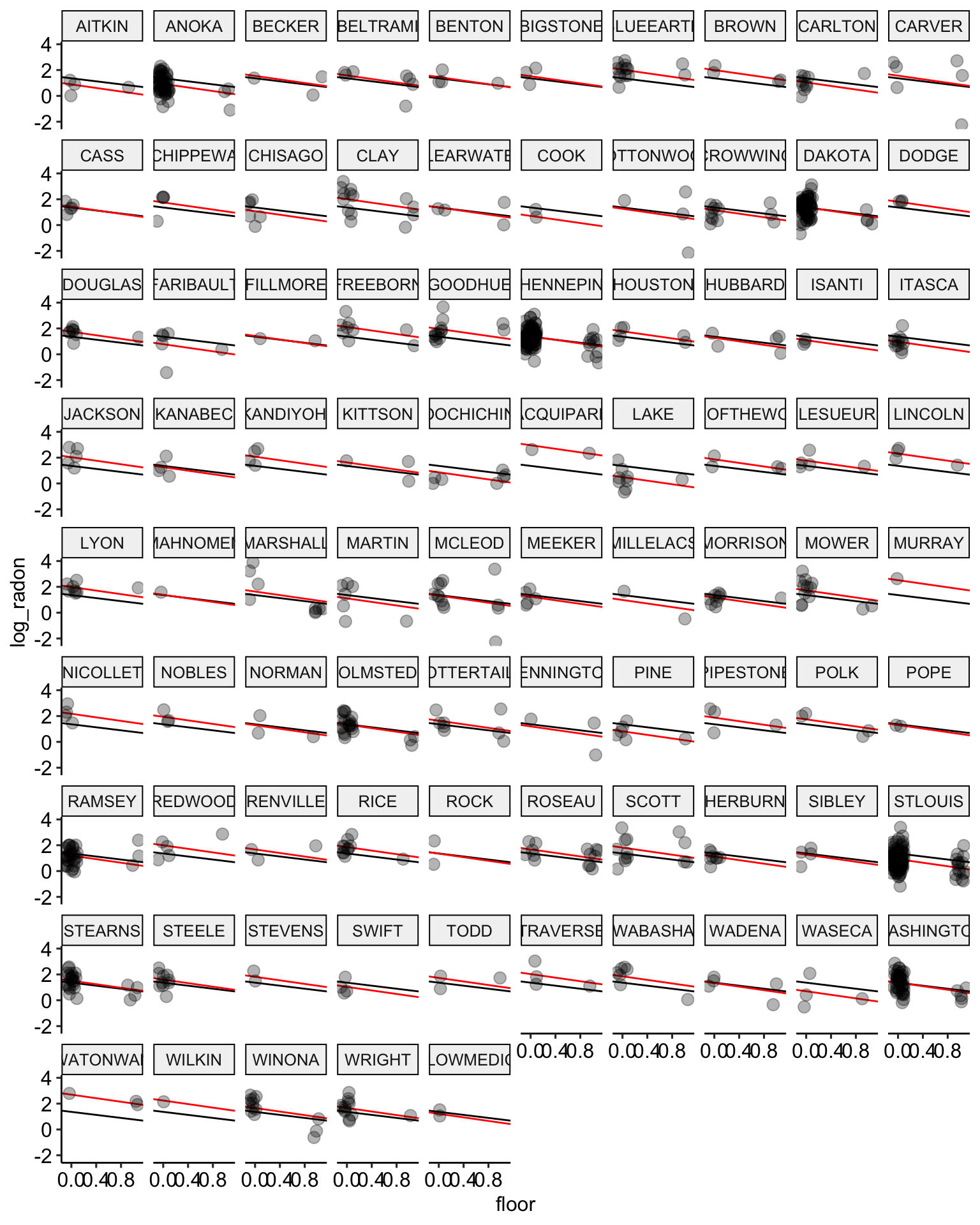
# plot the model results with posterior samples
stan.nopooling.samples <-
  stan.no.pooling.fit %>% # use this model fit
  recover_types(radon) %>%
  spread_draws(alpha[county], beta, sigma, n = 20) # extract 20 samples in tidy format

ggplot() +
  geom_abline(data = stan.pooling.samples,
            aes(intercept = alpha, slope = beta),
            color = "black",
            alpha = 0.3) +
  geom_abline(data = stan.nopooling.samples,
            aes(intercept = alpha, slope = beta),
            color = "red",
            alpha = 0.3) +
  geom_point(data = radon,
             aes(x = floor, y = log_radon, group = county),
             alpha = 0.3,
             size = 3,
             position = position_jitter(width = 0.1, height = 0.2)) +
  facet_wrap(~ county) +
  ggpubr::theme_pubr()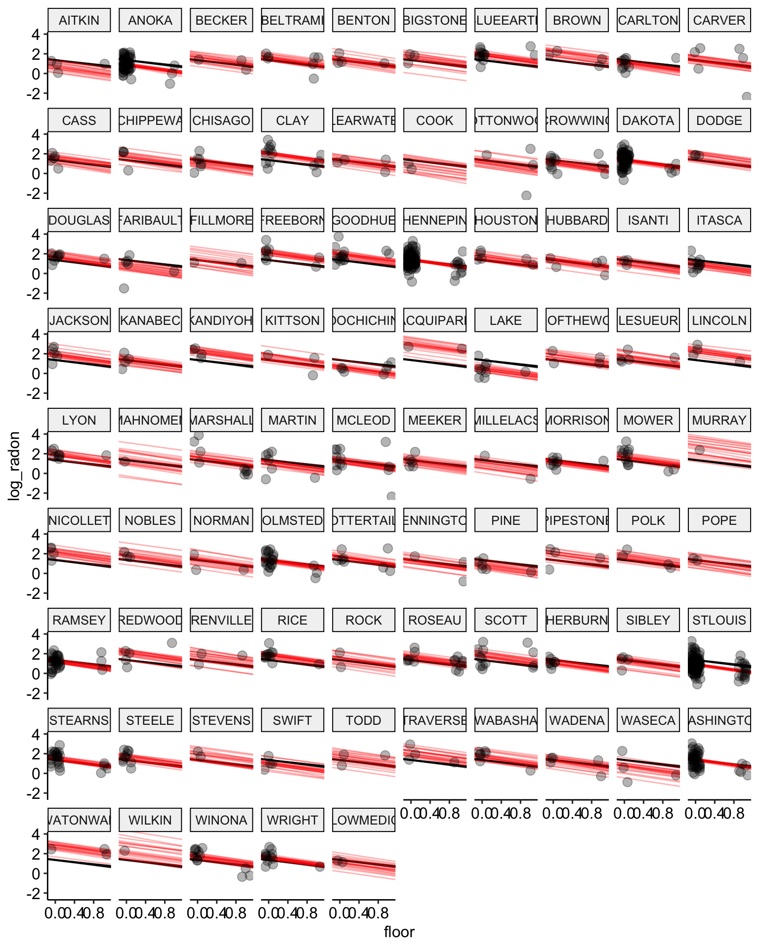
Partial Pooling
Now lets use a partial pooling model to estimate the relationship between a floor measurement and log radon level. As opposed to no pooling models, which essentially estimate a separate regression for each group, partial pooling models use information about the variance between groups get produce more accurate estimates for units within groups. So, for example, in counties were there are only 2 observations the partial pooling model will pull the floor estimates towards the mean of the full sample. This leads to less over fitting and more accurate predictions. Partial pooling models are more commonly known as multilevel or hierarchical models.
Frequentist Fit
Let’s fit the partial pooling model in a frequentist framework:
library(lme4)

# fit the model
partial.pooling.fit <- lmer(formula = log_radon ~ floor + (1 | county),
                            data = radon)

# print results
tidy(partial.pooling.fit, conf.int = TRUE)
## # A tibble: 4 × 8
## effect group term estimate std.error statistic conf.low conf.high
## <chr> <chr> <chr> <dbl> <dbl> <dbl> <dbl> <dbl>
## 1 fixed <NA> (Int… 1.49 0.0496 30.1 1.40 1.59
## 2 fixed <NA> floor -0.663 0.0677 -9.80 -0.795 -0.530
## 3 ran_pars coun… sd__… 0.315 NA NA NA NA
## 4 ran_pars Resi… sd__… 0.726 NA NA NA NA# calculate fitted values
radon$partial.pooling.fit <- fitted(partial.pooling.fit)
# plot the model results
ggplot(data = radon, aes(x = as_factor(floor), y = log_radon, group = county)) +
geom_line(aes(y = pooling.fit), color = "black") +
geom_line(aes(y = no.pooling.fit), color = "red") + # add no pooling estimates
geom_line(aes(y = partial.pooling.fit), color = "blue") + # add partial pooling estimates
geom_point(alpha = 0.3,
size = 3,
position = position_jitter(width = 0.1, height = 0.2)) +
facet_wrap(~ county) +
ggpubr::theme_pubr()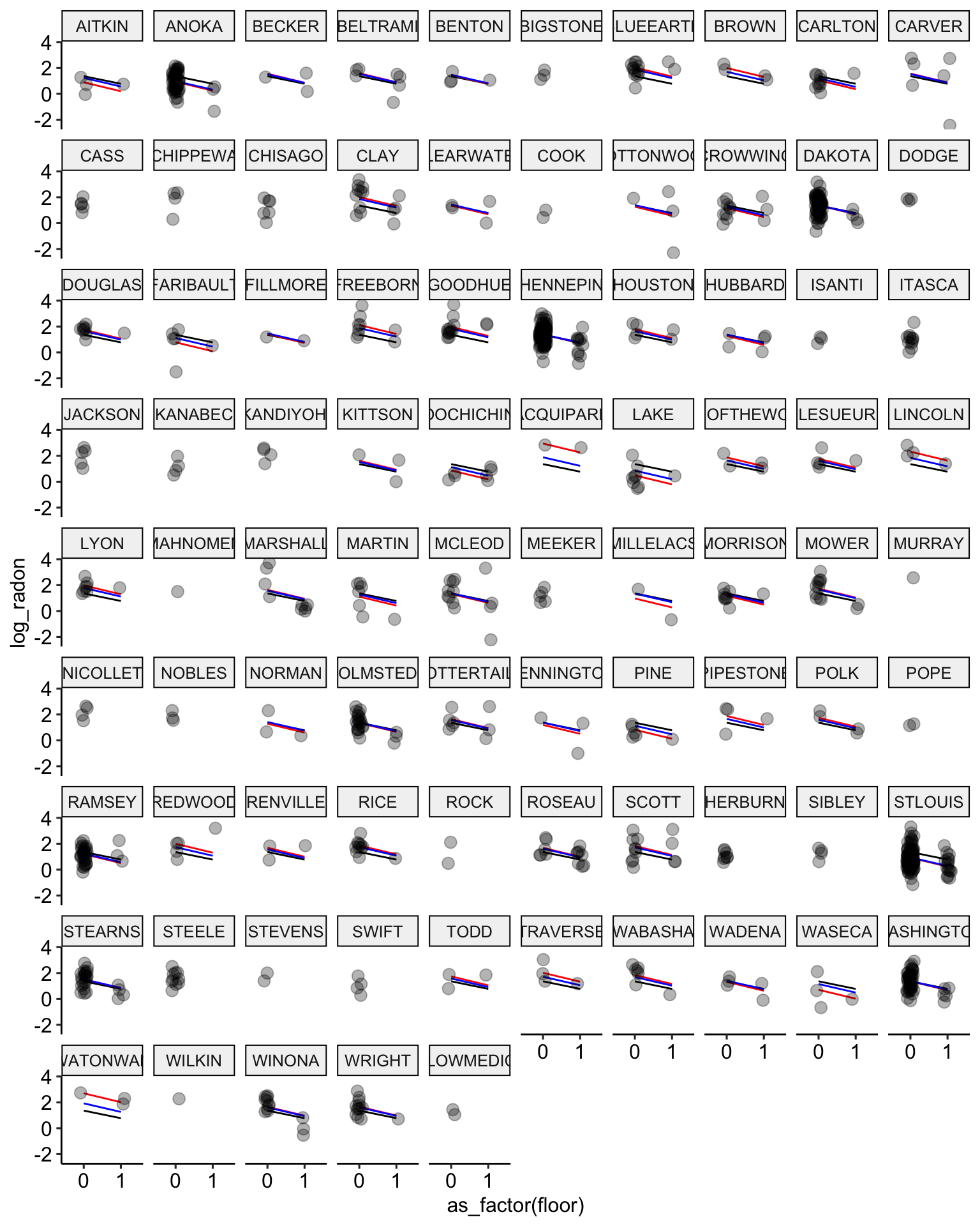
Bayesian Fit
Program the model in Stan.
data {
  int n; // number of observations
  int n_county; // number of counties
  vector[n] log_radon;
  vector[n] vfloor;
  int<lower = 0, upper = n_county> county[n];
}

parameters {
  vector[n_county] alpha; // vector of county intercepts
  real beta; // slope parameter
  real<lower = 0> sigma_a; // variance of counties
  real<lower = 0> sigma_y; // model residual variance
  real mu_a; // mean of counties
}

model {
  // conditional mean
  vector[n] mu;

  // linear combination
  mu = alpha[county] + beta * vfloor;

  // priors
  beta ~ normal(0, 1);

  // hyper-priors
  mu_a ~ normal(0, 1);
  sigma_a ~ cauchy(0, 2.5);
  sigma_y ~ cauchy(0, 2.5);

  // level-2 likelihood
  alpha ~ normal(mu_a, sigma_a);

  // level-1 likelihood
  log_radon ~ normal(mu, sigma_y);
}

generated quantities {
  vector[n] log_lik; // calculate log-likelihood
  vector[n] y_rep; // replications from posterior predictive distribution

  for (i in 1:n) {
    // generate mpg predicted value
    real log_radon_hat = alpha[county[i]] + beta * vfloor[i];

    // calculate log-likelihood
    log_lik[i] = normal_lpdf(log_radon[i] | log_radon_hat, sigma_y);
    // normal_lpdf is the log of the normal probability density function

    // generate replication values
    y_rep[i] = normal_rng(log_radon_hat, sigma_y);
    // normal_rng generates random numbers from a normal distribution
  }
}
Now we fit this model:
# prepare data for stan
model.data <-
  radon %>%
  rename(vfloor = floor) %>%
  dplyr::select(log_radon, vfloor, county) %>%
  compose_data()

# fit stan model
stan.partial.pooling.fit <- partial.pooling.model$sample(data = model.data,
                                                         refresh = 0)
## Running MCMC with 4 sequential chains...
##
## Chain 1 finished in 1.1 seconds.
## Chain 2 finished in 1.1 seconds.
## Chain 3 finished in 1.1 seconds.
## Chain 4 finished in 1.1 seconds.
##
## All 4 chains finished successfully.
## Mean chain execution time: 1.1 seconds.
## Total execution time: 4.7 seconds.rstan.stan.partial.pooling.fit <- read_stan_csv(stan.partial.pooling.fit$output_files())
tidy(rstan.stan.partial.pooling.fit, conf.int = TRUE)## # A tibble: 1,927 × 5
## term estimate std.error conf.low conf.high
## <chr> <dbl> <dbl> <dbl> <dbl>
## 1 alpha[1] 1.23 0.244 0.738 1.70
## 2 alpha[2] 0.983 0.0954 0.802 1.17
## 3 alpha[3] 1.50 0.249 1.02 1.99
## 4 alpha[4] 1.53 0.206 1.13 1.94
## 5 alpha[5] 1.47 0.240 0.992 1.94
## 6 alpha[6] 1.51 0.256 0.982 2.00
## 7 alpha[7] 1.87 0.164 1.56 2.19
## 8 alpha[8] 1.70 0.239 1.25 2.19
## 9 alpha[9] 1.20 0.184 0.830 1.56
## 10 alpha[10] 1.52 0.215 1.09 1.93
## # … with 1,917 more rowsstan.partialpool.values <-
stan.partial.pooling.fit %>% # use this model fit
recover_types(radon) %>% # this matches indexes to original factor levels
spread_draws(alpha[county], beta, sigma_a, sigma_y) %>% # extract samples in tidy format
median_hdci() # calculate the median HDCI
# plot the model results for the median estimates
ggplot(data = radon, aes(x = floor, y = log_radon, group = county)) +
geom_abline(data = stan.pooling.values,
aes(intercept = alpha, slope = beta), color = "black") +
# no pooling estimates in red
geom_abline(data = stan.nopool.values,
aes(intercept = alpha, slope = beta), color = "red") +
# partial pooling estimates in blue
geom_abline(data = stan.partialpool.values,
aes(intercept = alpha, slope = beta), color = "blue") +
geom_point(alpha = 0.3,
size = 3,
position = position_jitter(width = 0.1, height = 0.2)) +
facet_wrap(~ county) +
scale_color_manual(values = c("No Pooling", "Pooling")) +
ggpubr::theme_pubr()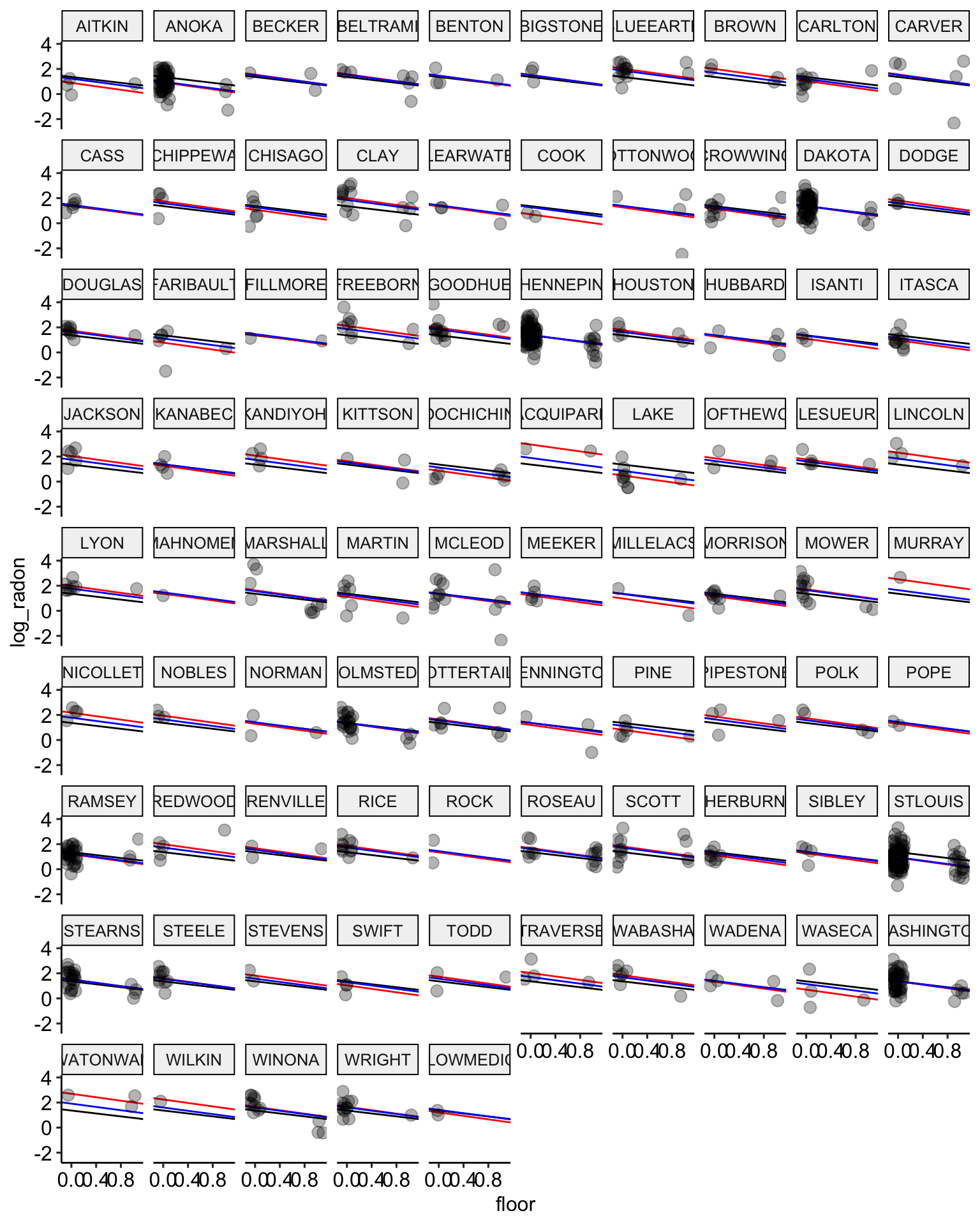
# plot the model results with posterior samples
stan.partialpool.samples <-
  stan.partial.pooling.fit %>% # use this model fit
  recover_types(radon) %>%
  spread_draws(alpha[county], beta, sigma_a, sigma_y, n = 20) # extract 20 samples in tidy format

ggplot() +
  geom_abline(data = stan.pooling.samples,
            aes(intercept = alpha, slope = beta),
            color = "black",
            alpha = 0.3) +
  geom_abline(data = stan.nopooling.samples,
            aes(intercept = alpha, slope = beta),
            color = "red",
            alpha = 0.3) +
  geom_abline(data = stan.partialpool.samples,
            aes(intercept = alpha, slope = beta),
            color = "blue",
            alpha = 0.3) +
  geom_point(data = radon,
             aes(x = floor, y = log_radon, group = county),
             alpha = 0.3,
             size = 3,
             position = position_jitter(width = 0.1, height = 0.2)) +
  facet_wrap(~ county) +
  ggpubr::theme_pubr()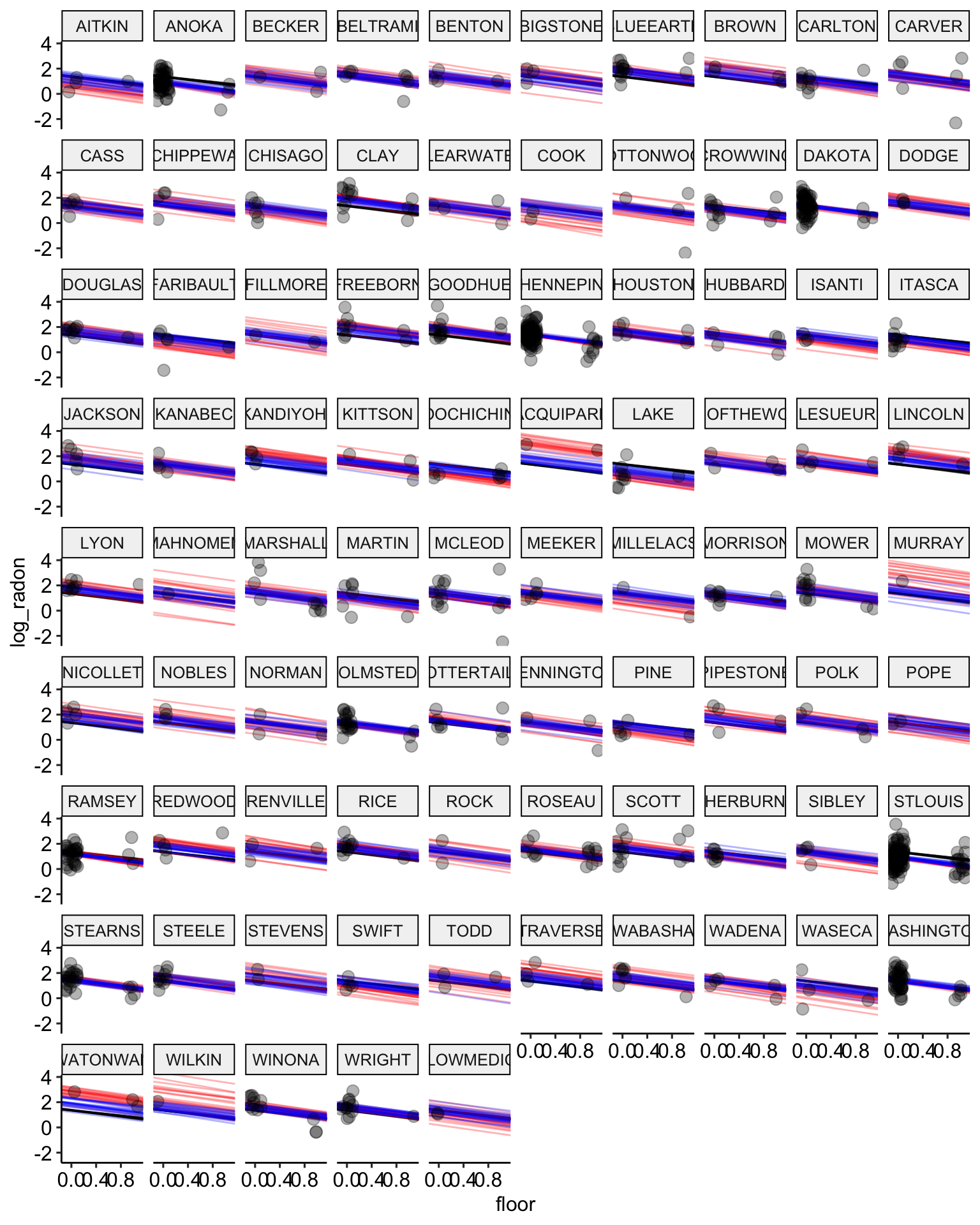
Adding Group-level Predictors
Partial pooling also allow us to include group-level predictor variables which can dramatically improve the model’s predictions. Let’s add a group-level predictor to the model. For a group-level predictor, let’s add a measure of the county’s uranium level.
Frequentist Fit
In frequentist, we can fit this model as follows:
# fit model
partial.pooling.fit.02 <- lmer(formula = log_radon ~ floor + log_uranium + (1 | county),
                               data = radon)

# print model results
tidy(partial.pooling.fit.02, conf.int = TRUE)
## # A tibble: 5 × 8
## effect group term estimate std.error statistic conf.low conf.high
## <chr> <chr> <chr> <dbl> <dbl> <dbl> <dbl> <dbl>
## 1 fixed <NA> (Int… 1.50 0.0362 41.3 1.43 1.57
## 2 fixed <NA> floor -0.639 0.0660 -9.67 -0.768 -0.509
## 3 fixed <NA> log_… 0.697 0.0876 7.96 0.526 0.869
## 4 ran_pars coun… sd__… 0.148 NA NA NA NA
## 5 ran_pars Resi… sd__… 0.728 NA NA NA NA# calculate fitted values
radon$partial.pooling.fit.02 <- fitted(partial.pooling.fit.02)
# plot the model results
ggplot(data = radon, aes(x = as_factor(floor), y = log_radon, group = county)) +
geom_line(aes(y = pooling.fit), color = "black") +
geom_line(aes(y = no.pooling.fit), color = "red") + # add no pooling estimates
# partial pooling with group-level predictor in dashed purple
geom_line(aes(y = partial.pooling.fit.02), color = "purple", lty = 2) +
# partial pooling without group-level predictors in blue
geom_line(aes(y = partial.pooling.fit), color = "blue") + # add partial pooling estimates
geom_point(alpha = 0.3,
size = 3,
position = position_jitter(width = 0.1, height = 0.2)) +
facet_wrap(~ county) +
ggpubr::theme_pubr()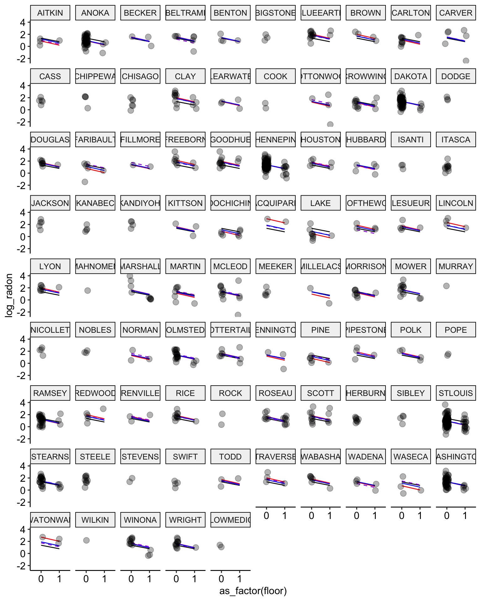
Bayesian Fit
To program this model in Stan, we’ll use the transformed parameters block to create a conditional mean equation for the level 2 model.
data {
  int n; // number of observations
  int n_county; // number of counties
  vector[n] log_radon;
  vector[n] vfloor;
  vector[n] log_uranium;
  int<lower = 0, upper = n_county> county[n];
}

parameters {
  vector[n_county] alpha; // vector of county intercepts
  real b_floor; // slope parameter
  real b_uranium;
  real<lower = 0> sigma_a; // variance of counties
  real<lower = 0> sigma_y; // model residual variance
  real mu_a; // mean of counties
}

model {
  // conditional mean
  vector[n] mu;

  // linear combination
  mu = alpha[county] + b_floor * vfloor + b_uranium * log_uranium;

  // priors
  b_floor ~ normal(0, 100);
  b_uranium ~ normal(0, 100);

  // hyper-priors
  mu_a ~ normal(0, 10);
  sigma_a ~ cauchy(0, 2.5);
  sigma_y ~ cauchy(0, 2.5);

  // level-2 likelihood
  alpha ~ normal(mu_a, sigma_a);

  // level-1 likelihood
  log_radon ~ normal(mu, sigma_y);
}

generated quantities {
  vector[n] log_lik; // calculate log-likelihood
  vector[n] y_rep; // replications from posterior predictive distribution

  for (i in 1:n) {
    // generate mpg predicted value
    real log_radon_hat = alpha[county[i]] + b_floor * vfloor[i] + b_uranium * log_uranium[i];

    // calculate log-likelihood
    log_lik[i] = normal_lpdf(log_radon[i] | log_radon_hat, sigma_y);
    // normal_lpdf is the log of the normal probability density function

    // generate replication values
    y_rep[i] = normal_rng(log_radon_hat, sigma_y);
    // normal_rng generates random numbers from a normal distribution
  }
}
Now we fit this model:
# prepare data for stan
model.data <-
  radon %>%
  rename(vfloor = floor) %>%
  dplyr::select(log_radon, vfloor, county, log_uranium) %>%
  compose_data()

# fit stan model
stan.partial.pooling.model.02 <- partial.pooling.model.02$sample(data = model.data,
                                                                 refresh = 0)
## Running MCMC with 4 sequential chains...
##
## Chain 1 finished in 1.6 seconds.
## Chain 2 finished in 1.6 seconds.
## Chain 3 finished in 1.7 seconds.
## Chain 4 finished in 1.6 seconds.
##
## All 4 chains finished successfully.
## Mean chain execution time: 1.6 seconds.
## Total execution time: 7.0 seconds.rstan.stan.partial.pooling.fit.02 <- read_stan_csv(stan.partial.pooling.model.02$output_files())
tidy(rstan.stan.partial.pooling.fit.02, conf.int = TRUE)## # A tibble: 1,928 × 5
## term estimate std.error conf.low conf.high
## <chr> <dbl> <dbl> <dbl> <dbl>
## 1 alpha[1] 1.47 0.145 1.17 1.76
## 2 alpha[2] 1.51 0.0976 1.32 1.71
## 3 alpha[3] 1.50 0.148 1.22 1.83
## 4 alpha[4] 1.58 0.150 1.36 1.93
## 5 alpha[5] 1.50 0.146 1.22 1.81
## 6 alpha[6] 1.47 0.142 1.17 1.75
## 7 alpha[7] 1.60 0.131 1.39 1.90
## 8 alpha[8] 1.52 0.145 1.27 1.84
## 9 alpha[9] 1.43 0.132 1.15 1.68
## 10 alpha[10] 1.49 0.141 1.21 1.78
## # … with 1,918 more rowsstan.partialpool.02.values <-
stan.partial.pooling.model.02 %>% # use this model fit
recover_types(radon) %>% # this matches indexes to original factor levels
spread_draws(alpha[county], b_floor, b_uranium, sigma_a, sigma_y) %>% # extract samples in tidy format
median_hdci() # calculate the median HDCI
# plot the model results for the median estimates
ggplot(data = radon, aes(x = floor, y = log_radon, group = county)) +
geom_abline(data = stan.pooling.values,
aes(intercept = alpha, slope = beta), color = "black") +
# no pooling estimates in red
geom_abline(data = stan.nopool.values,
aes(intercept = alpha, slope = beta), color = "red") +
# partial pooling estimates in blue
geom_abline(data = stan.partialpool.values,
aes(intercept = alpha, slope = beta), color = "blue") +
geom_abline(data = stan.partialpool.02.values,
aes(intercept = alpha, slope = b_floor), color = "purple", lty = 2) +
geom_point(alpha = 0.3,
size = 3,
position = position_jitter(width = 0.1, height = 0.2)) +
facet_wrap(~ county) +
scale_color_manual(values = c("No Pooling", "Pooling")) +
ggpubr::theme_pubr()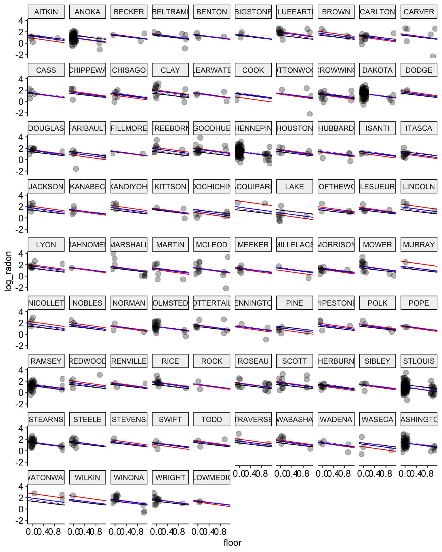
# plot the model results with posterior samples
stan.partialpool.02.samples <-
  stan.partial.pooling.model.02 %>% # use this model fit
  recover_types(radon) %>%
  spread_draws(alpha[county], b_floor, b_uranium, sigma_a, sigma_y, n = 20) # extract 20 samples in tidy format

ggplot() +
  geom_abline(data = stan.pooling.samples,
            aes(intercept = alpha, slope = beta),
            color = "black",
            alpha = 0.3) +
  geom_abline(data = stan.nopooling.samples,
            aes(intercept = alpha, slope = beta),
            color = "red",
            alpha = 0.3) +
  geom_abline(data = stan.partialpool.samples,
            aes(intercept = alpha, slope = beta),
            color = "blue",
            alpha = 0.3) +
  geom_abline(data = stan.partialpool.02.samples,
            aes(intercept = alpha, slope = b_floor),
            color = "purple",
            lty = 2,
            alpha = 0.3) +
  geom_point(data = radon,
             aes(x = floor, y = log_radon, group = county),
             alpha = 0.3,
             size = 3,
             position = position_jitter(width = 0.1, height = 0.2)) +
  facet_wrap(~ county) +
  ggpubr::theme_pubr()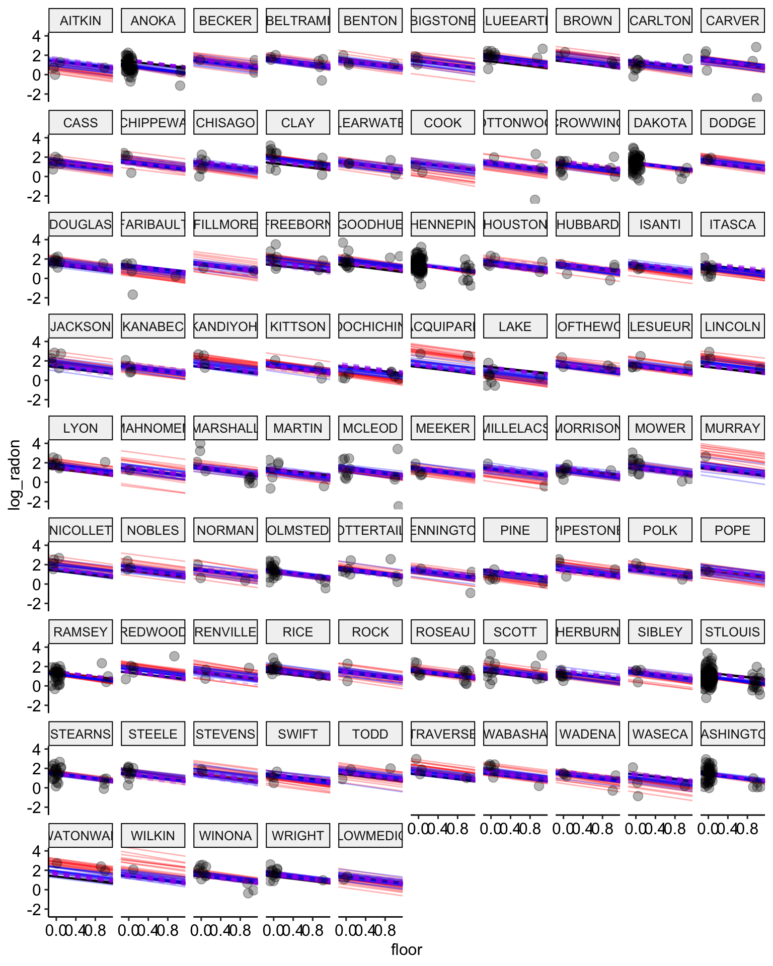
Varying Slope Model
There’s no reason that we need to estimate the same slope for every county, and partial pooling models allow us to let the slopes parameters vary between counties. Let’s estimate a final model where we let the effect of floor vary between counties.
Frequentist Fit
# fit model
partial.pooling.fit.03 <- lmer(formula = log_radon ~ floor + log_uranium +
                                 (1 + floor | county),
                               data = radon)

# print model results
tidy(partial.pooling.fit.03, conf.int = TRUE)
## # A tibble: 7 × 8
## effect group term estimate std.error statistic conf.low conf.high
## <chr> <chr> <chr> <dbl> <dbl> <dbl> <dbl> <dbl>
## 1 fixed <NA> (Int… 1.49 0.0341 43.8 1.43 1.56
## 2 fixed <NA> floor -0.615 0.0838 -7.34 -0.779 -0.451
## 3 fixed <NA> log_… 0.745 0.0849 8.77 0.578 0.911
## 4 ran_pars coun… sd__… 0.122 NA NA NA NA
## 5 ran_pars coun… cor_… 0.204 NA NA NA NA
## 6 ran_pars coun… sd__… 0.342 NA NA NA NA
## 7 ran_pars Resi… sd__… 0.719 NA NA NA NA# calculate fitted values
radon$partial.pooling.fit.03 <- fitted(partial.pooling.fit.03)
# plot the model results
ggplot(data = radon, aes(x = as_factor(floor), y = log_radon, group = county)) +
geom_line(aes(y = pooling.fit), color = "black") +
geom_line(aes(y = no.pooling.fit), color = "red") + # add no pooling estimates
# partial pooling with group-level predictor in dashed purple
geom_line(aes(y = partial.pooling.fit.02), color = "purple", lty = 2) +
# partial pooling without group-level predictors in blue
geom_line(aes(y = partial.pooling.fit), color = "blue") + # add partial pooling estimates
geom_line(aes(y = partial.pooling.fit.03), color = "green") +
geom_point(alpha = 0.3,
size = 3,
position = position_jitter(width = 0.1, height = 0.2)) +
facet_wrap(~ county) +
ggpubr::theme_pubr()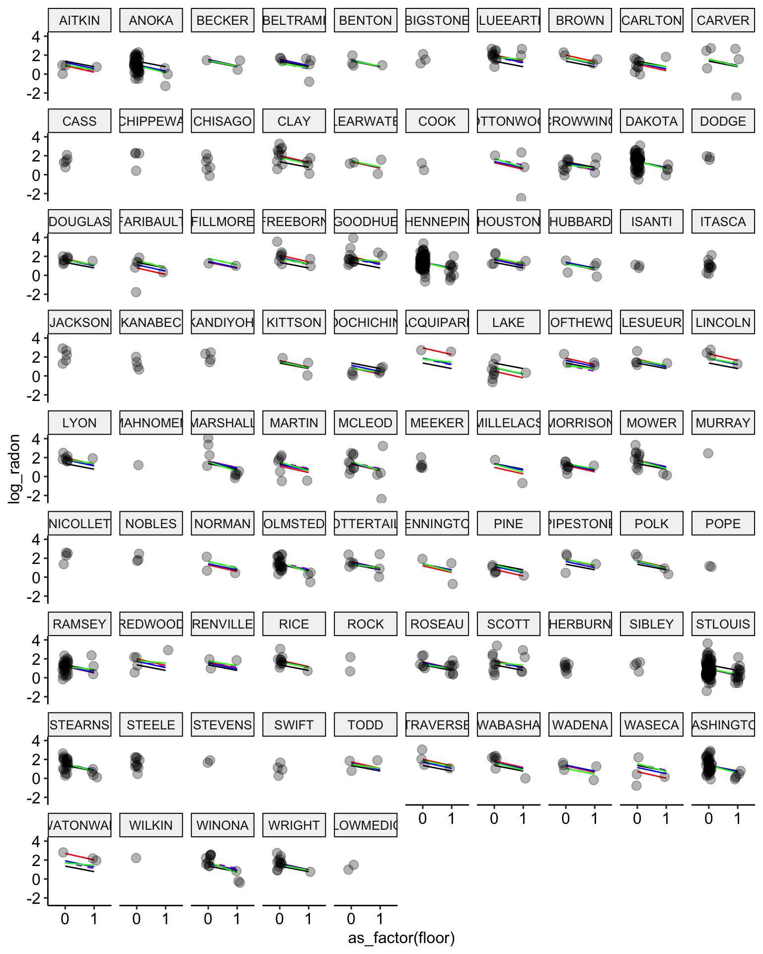
Bayesian Fit
To program this model in Stan, we’ll need to include the variance covariance matrix for the varying intercept and slope parameters.
data {
  int n; // number of observations
  int n_county; // number of counties
  int<lower = 0, upper = n_county> county[n];

  // level 1 variables
  vector[n] log_radon;
  int vfloor[n];

  // level 2 variables
  real log_uranium[n];
}

parameters {
  vector[n_county] b_floor;
  vector[n_county] a_county;
  real b_uranium;
  real a;
  real b;
  vector<lower=0>[2] sigma_county;
  real<lower=0> sigma;
  corr_matrix[2] Rho;
}

model {
  // conditional mean
  vector[n] mu;

  // varying slopes and varying intercepts component
  {
  // vector for intercept mean and slope mean
  vector[2] YY[n_county];
  vector[2] MU;
  MU = [a , b]';
  for (j in 1:n_county) YY[j] = [a_county[j], b_floor[j]]';
    YY ~ multi_normal(MU , quad_form_diag(Rho , sigma_county));
  }

  // linear model
  for (i in 1:n) {
    mu[i] = a_county[county[i]] + b_floor[county[i]] * vfloor[i] + b_uranium * log_uranium[i];
  }

  // priors
  sigma ~ exponential(3);
  b_uranium ~ normal(0 , 100);

  // hyper-priors
  Rho ~ lkj_corr(1);
  sigma_county ~ exponential(3);
  b ~ normal(0 , 100);
  a ~ normal(0 , 100);

  // likelihood
  log_radon ~ normal(mu , sigma);
}

generated quantities {
  vector[n] log_lik; // calculate log-likelihood
  vector[n] y_rep; // replications from posterior predictive distribution

  for (i in 1:n) {
    // generate mpg predicted value
    real log_radon_hat = a_county[county[i]] + b_floor[county[i]] * vfloor[i] + b_uranium * log_uranium[i];

    // calculate log-likelihood
    log_lik[i] = normal_lpdf(log_radon[i] | log_radon_hat, sigma);
    // normal_lpdf is the log of the normal probability density function

    // generate replication values
    y_rep[i] = normal_rng(log_radon_hat, sigma);
    // normal_rng generates random numbers from a normal distribution
  }
}
Now we fit this model:
# prepare data for stan
model.data <-
  radon %>%
  rename(vfloor = floor) %>%
  dplyr::select(log_radon, vfloor, county, log_uranium) %>%
  compose_data()

# fit stan model
stan.partial.pooling.model.03 <- partial.pooling.model.03$sample(data = model.data,
                                                                 refresh = 0)
## Running MCMC with 4 sequential chains...
##
## Chain 1 finished in 17.3 seconds.
## Chain 2 finished in 5.5 seconds.
## Chain 3 finished in 7.0 seconds.
## Chain 4 finished in 5.5 seconds.
##
## All 4 chains finished successfully.
## Mean chain execution time: 8.8 seconds.
## Total execution time: 35.8 seconds.rstan.stan.partial.pooling.fit.03 <- read_stan_csv(stan.partial.pooling.model.03$output_files())
tidy(rstan.stan.partial.pooling.fit.03, conf.int = TRUE)## # A tibble: 2,018 × 5
## term estimate std.error conf.low conf.high
## <chr> <dbl> <dbl> <dbl> <dbl>
## 1 b_floor[1] -0.578 0.275 -1.07 0.0620
## 2 b_floor[2] -0.696 0.246 -1.27 -0.266
## 3 b_floor[3] -0.603 0.247 -1.09 -0.0606
## 4 b_floor[4] -0.509 0.231 -0.939 -0.00409
## 5 b_floor[5] -0.580 0.273 -1.09 0.0265
## 6 b_floor[6] -0.636 0.299 -1.23 0.00619
## 7 b_floor[7] -0.398 0.292 -0.828 0.309
## 8 b_floor[8] -0.604 0.243 -1.07 -0.0826
## 9 b_floor[9] -0.529 0.298 -0.974 0.236
## 10 b_floor[10] -0.688 0.241 -1.22 -0.245
## # … with 2,008 more rowsstan.partialpool.03.values <-
stan.partial.pooling.model.03 %>% # use this model fit
recover_types(radon) %>% # this matches indexes to original factor levels
spread_draws(a_county[county], b_floor[county], b_uranium, sigma_county[], sigma) %>% # extract samples in tidy format
median_hdci() # calculate the median HDCI
# plot the model results for the median estimates
ggplot(data = radon, aes(x = floor, y = log_radon, group = county)) +
geom_abline(data = stan.pooling.values,
aes(intercept = alpha, slope = beta), color = "black") +
# no pooling estimates in red
geom_abline(data = stan.nopool.values,
aes(intercept = alpha, slope = beta), color = "red") +
# partial pooling estimates in blue
geom_abline(data = stan.partialpool.values,
aes(intercept = alpha, slope = beta), color = "blue") +
geom_abline(data = stan.partialpool.02.values,
aes(intercept = alpha, slope = b_floor), color = "purple", lty = 2) +
geom_abline(data = stan.partialpool.03.values,
aes(intercept = a_county, slope = b_floor), color = "green") +
geom_point(alpha = 0.3,
size = 3,
position = position_jitter(width = 0.1, height = 0.2)) +
facet_wrap(~ county) +
scale_color_manual(values = c("No Pooling", "Pooling")) +
ggpubr::theme_pubr()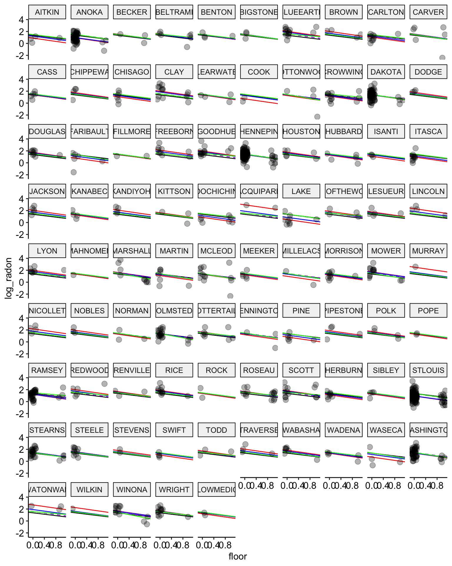
# plot the model results with posterior samples
stan.partialpool.03.samples <-
  stan.partial.pooling.model.03 %>% # use this model fit
  recover_types(radon) %>%
  spread_draws(a_county[county], b_floor[county], b_uranium, sigma_county[], sigma, n = 20) # extract 20 samples in tidy format

ggplot() +
  geom_abline(data = stan.pooling.samples,
            aes(intercept = alpha, slope = beta),
            color = "black",
            alpha = 0.3) +
  geom_abline(data = stan.nopooling.samples,
            aes(intercept = alpha, slope = beta),
            color = "red",
            alpha = 0.3) +
  geom_abline(data = stan.partialpool.samples,
            aes(intercept = alpha, slope = beta),
            color = "blue",
            alpha = 0.3) +
  geom_abline(data = stan.partialpool.02.samples,
            aes(intercept = alpha, slope = b_floor),
            color = "purple",
            lty = 2,
            alpha = 0.3) +
  geom_abline(data = stan.partialpool.03.samples,
            aes(intercept = a_county, slope = b_floor),
            color = "green",
            alpha = 0.3) +
  geom_point(data = radon,
             aes(x = floor, y = log_radon, group = county),
             alpha = 0.3,
             size = 3,
             position = position_jitter(width = 0.1, height = 0.2)) +
  facet_wrap(~ county) +
  ggpubr::theme_pubr()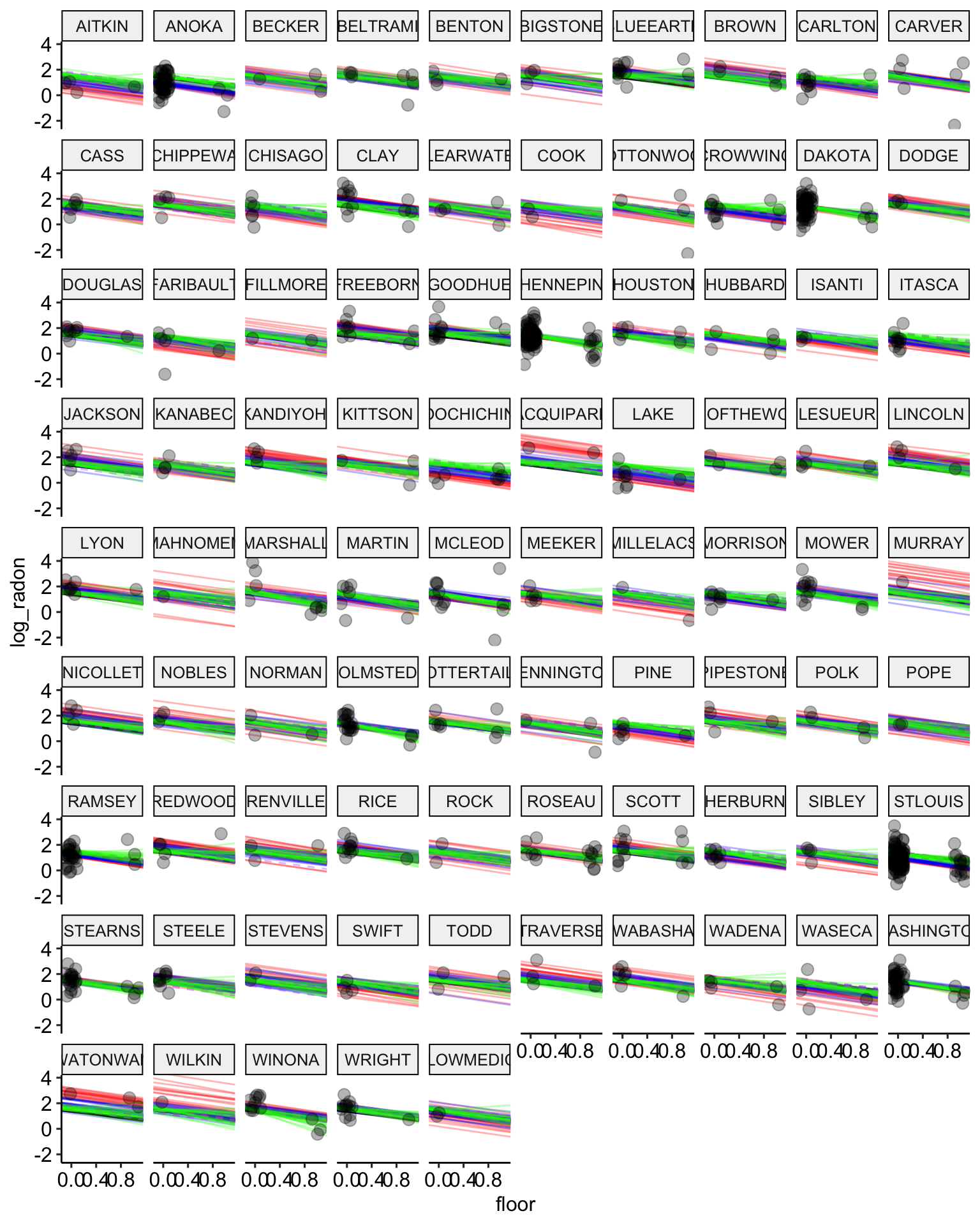
Model Comparison
Now we can compute the widely applicable information criterion (WAIC) to determine which has the best fit to the data:
library(rethinking)

compare(stan.pooling.fit, rstan.stan.no.pooling.fit,
        rstan.stan.partial.pooling.fit, rstan.stan.partial.pooling.fit.02,
        rstan.stan.partial.pooling.fit.03)
## WAIC SE dWAIC
## rstan.stan.partial.pooling.fit.02 2054.615 57.54352 0.000000
## rstan.stan.partial.pooling.fit.03 2057.063 59.36121 2.447496
## rstan.stan.partial.pooling.fit 2071.685 55.83546 17.069744
## rstan.stan.no.pooling.fit 2118.367 56.46214 63.751704
## stan.pooling.fit 2179.970 49.92133 125.354529
## dSE pWAIC weight
## rstan.stan.partial.pooling.fit.02 NA 25.974319 7.726052e-01
## rstan.stan.partial.pooling.fit.03 6.046955 43.977915 2.272430e-01
## rstan.stan.partial.pooling.fit 10.460089 48.051214 1.518133e-04
## rstan.stan.no.pooling.fit 17.726772 83.018908 1.107774e-14
## stan.pooling.fit 23.387237 3.842781 4.651227e-28plot(compare(stan.pooling.fit, rstan.stan.no.pooling.fit,
rstan.stan.partial.pooling.fit, rstan.stan.partial.pooling.fit.02,
rstan.stan.partial.pooling.fit.03))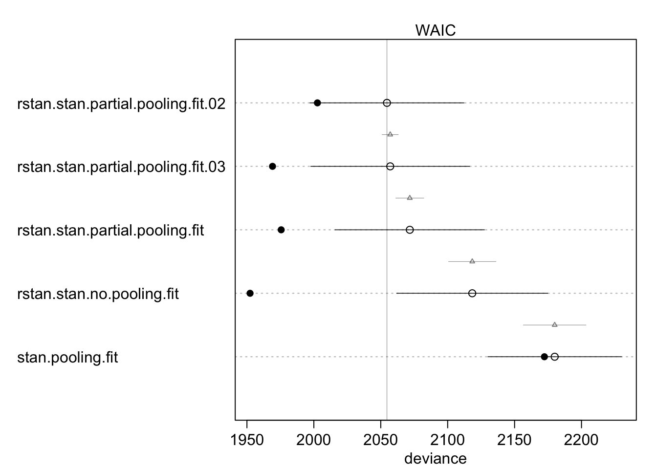
These results show that the stan.partial.pooling.model.02, which is the varying intercept with a group-level predictor, has the lowest WAIC. In other words, this model provides the best out-of-sample predictions. The varying intercept, varying slope model is very closely behind with and increase in WAIC of only 3.2 points. The plot shows that although the varying intercept model with a group-level predictor has the best out-of-sample performance (open dots), it does not have the best in-sample performance (solid dots). The no-pooling model has the best in-sample performance, but this model also has the largest degree of over fitting.