Linear Models in Stan
In this tutorial, we will learn how to estimate linear models using Stan and R. Along the way, we will review the steps in a sound Bayesian workflow. This workflow consists of:
Considering the social process that generates your data. The goal of your statistical model should be to model the data generating process, so think hard about this. Exploratory analysis goes a long way towards helping you to understand this process.
Program your statistical model and sample from it.
Evaluate your model’s reliability. Check for Markov chain convergence to make sure that your model has produced reliable estimates.
Evaluate your model’s performance. How well does your model approximate the data generating process? This involves using posterior predictive checks.
Summarize your model’s results in tabular and graphical form.
My goal is to explain the fundamentals of linear models in Stan with examples so that we aren’t learning Stan programming in such an abstract environment. Let’s get started!
Import Data
We’ll use the Motor Trend Car Road Tests mtcars data that is provided in R as our practice data set.
cars.data <- mtcars

library(tidyverse)
## ── Attaching packages ─────────────────────────────────────── tidyverse 1.3.1 ──## ✓ ggplot2 3.3.5 ✓ purrr 0.3.4
## ✓ tibble 3.1.6 ✓ dplyr 1.0.7
## ✓ tidyr 1.1.4 ✓ stringr 1.4.0
## ✓ readr 2.1.1 ✓ forcats 0.5.1## ── Conflicts ────────────────────────────────────────── tidyverse_conflicts() ──
## x dplyr::filter() masks stats::filter()
## x dplyr::lag() masks stats::lag()glimpse(cars.data)## Rows: 32
## Columns: 11
## $ mpg <dbl> 21.0, 21.0, 22.8, 21.4, 18.7, 18.1, 14.3, 24.4, 22.8, 19.2, 17.8,…
## $ cyl <dbl> 6, 6, 4, 6, 8, 6, 8, 4, 4, 6, 6, 8, 8, 8, 8, 8, 8, 4, 4, 4, 4, 8,…
## $ disp <dbl> 160.0, 160.0, 108.0, 258.0, 360.0, 225.0, 360.0, 146.7, 140.8, 16…
## $ hp <dbl> 110, 110, 93, 110, 175, 105, 245, 62, 95, 123, 123, 180, 180, 180…
## $ drat <dbl> 3.90, 3.90, 3.85, 3.08, 3.15, 2.76, 3.21, 3.69, 3.92, 3.92, 3.92,…
## $ wt <dbl> 2.620, 2.875, 2.320, 3.215, 3.440, 3.460, 3.570, 3.190, 3.150, 3.…
## $ qsec <dbl> 16.46, 17.02, 18.61, 19.44, 17.02, 20.22, 15.84, 20.00, 22.90, 18…
## $ vs <dbl> 0, 0, 1, 1, 0, 1, 0, 1, 1, 1, 1, 0, 0, 0, 0, 0, 0, 1, 1, 1, 1, 0,…
## $ am <dbl> 1, 1, 1, 0, 0, 0, 0, 0, 0, 0, 0, 0, 0, 0, 0, 0, 0, 1, 1, 1, 0, 0,…
## $ gear <dbl> 4, 4, 4, 3, 3, 3, 3, 4, 4, 4, 4, 3, 3, 3, 3, 3, 3, 4, 4, 4, 3, 3,…
## $ carb <dbl> 4, 4, 1, 1, 2, 1, 4, 2, 2, 4, 4, 3, 3, 3, 4, 4, 4, 1, 2, 1, 1, 2,…Let’s walk though what our variables are:
mpg: Miles pre galloncyl: Number of cylindersdispDisplacement (cu. in.)hp: Gross horsepowerdrat: Rear axle ratiowt: Weight (1000 lbs)qsec: 1/4 mile timevs: Engine (0 = V-shaped, 1 = straight)am: Transmission (0 = automatic, 1 = manual)gear: Number of forward gearscarb: Number of carburetors
With this information, let’s do some quick data cleaning.
cars.data <-
  cars.data %>%
  rename(cylinders = cyl,
         displacement = disp,
         rear_axle_ratio = drat,
         weight = wt,
         engine_type = vs,
         trans_type = am,
         gears = gear) %>%
  mutate(engine_type = factor(engine_type, levels = c(0, 1),
                              labels = c("V-shaped", "Straight")),
         trans_type = factor(trans_type, levels = c(0, 1),
                             labels = c("Automatic", "Manual")))

glimpse(cars.data)
## Rows: 32
## Columns: 11
## $ mpg <dbl> 21.0, 21.0, 22.8, 21.4, 18.7, 18.1, 14.3, 24.4, 22.8, …
## $ cylinders <dbl> 6, 6, 4, 6, 8, 6, 8, 4, 4, 6, 6, 8, 8, 8, 8, 8, 8, 4, …
## $ displacement <dbl> 160.0, 160.0, 108.0, 258.0, 360.0, 225.0, 360.0, 146.7…
## $ hp <dbl> 110, 110, 93, 110, 175, 105, 245, 62, 95, 123, 123, 18…
## $ rear_axle_ratio <dbl> 3.90, 3.90, 3.85, 3.08, 3.15, 2.76, 3.21, 3.69, 3.92, …
## $ weight <dbl> 2.620, 2.875, 2.320, 3.215, 3.440, 3.460, 3.570, 3.190…
## $ qsec <dbl> 16.46, 17.02, 18.61, 19.44, 17.02, 20.22, 15.84, 20.00…
## $ engine_type <fct> V-shaped, V-shaped, Straight, Straight, V-shaped, Stra…
## $ trans_type <fct> Manual, Manual, Manual, Automatic, Automatic, Automati…
## $ gears <dbl> 4, 4, 4, 3, 3, 3, 3, 4, 4, 4, 4, 3, 3, 3, 3, 3, 3, 4, …
## $ carb <dbl> 4, 4, 1, 1, 2, 1, 4, 2, 2, 4, 4, 3, 3, 3, 4, 4, 4, 1, …For our research question, we will be investigating how different characteristics of a car affect it’s MPG. To start with, we will test how vehicle weight affects MPG. Let’s do some preliminary analysis of this question with visualizations.
ggplot(data = cars.data, aes(x = weight, y = mpg)) +
  geom_point()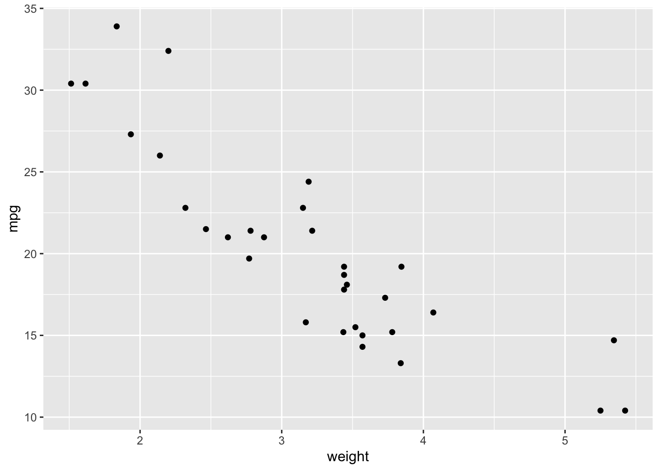
As expected, there seems to be a negative relationship between these variables. Let’s add in a fitted line:
ggplot(data = cars.data, aes(x = weight, y = mpg)) +
  geom_point() +
  geom_smooth(method = "lm")
## `geom_smooth()` using formula 'y ~ x'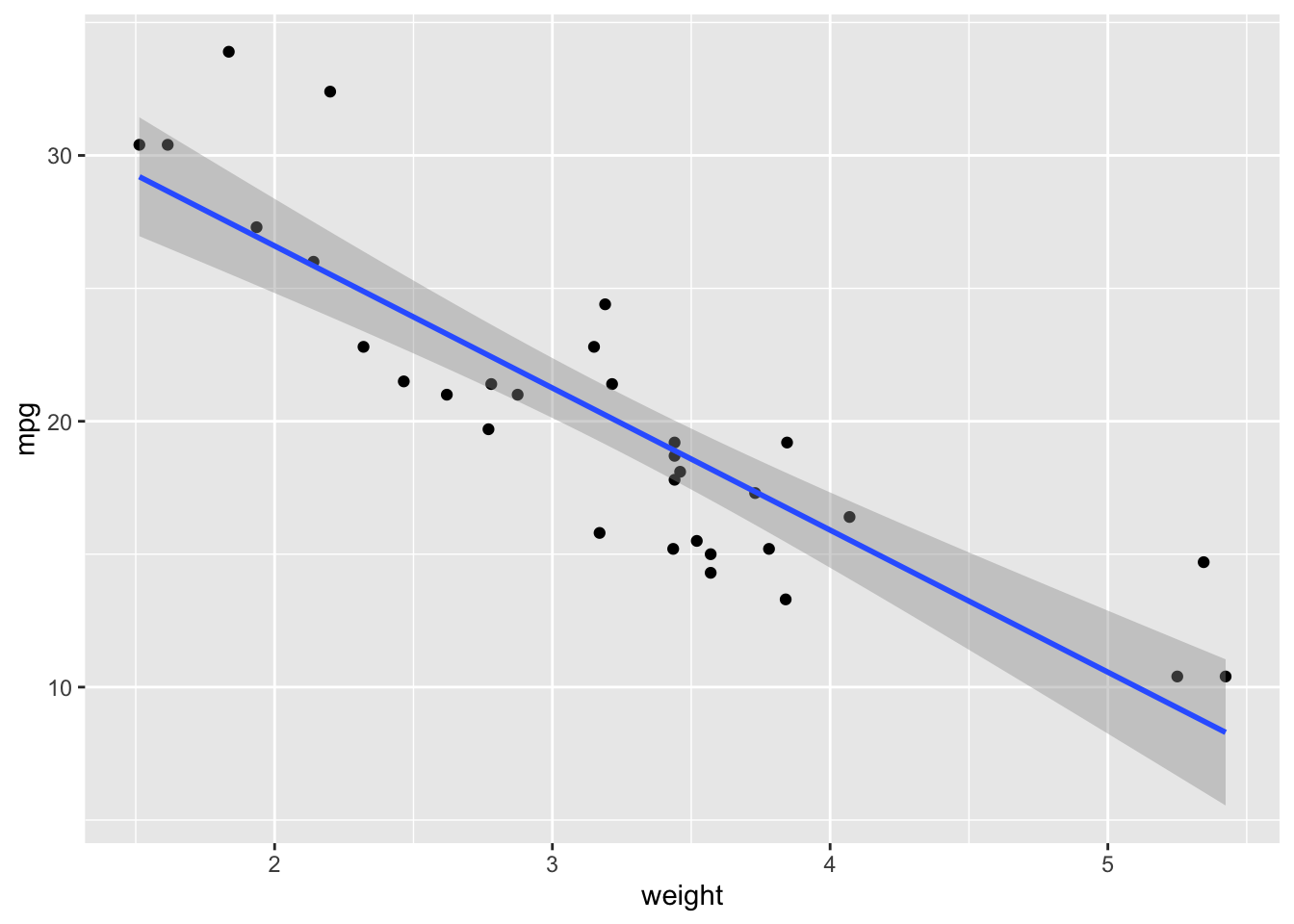
Build a Model
Models with a Single Predictor
Now we will build a model in Stan to formally estimate this relationship. Rather than creating an r code block, we want to create a stan code block. The only caveat is that we also need to add a name for our Stan model provided in the output.var argument.
Here is the model that we want to estimate in Stan:
\[ \begin{aligned} \text{mpg} &\sim \text{Normal}(\mu, \sigma) \\ \mu &= \alpha + \beta \text{weight} \end{aligned} \]
To start, we need to load cmdstanr which will allow us to interface with Stan through R.
library(cmdstanr)## This is cmdstanr version 0.4.0## - Online documentation and vignettes at mc-stan.org/cmdstanr## - CmdStan path set to: /Users/nickjenkins/.cmdstanr/cmdstan-2.28.1## - Use set_cmdstan_path() to change the path##
## A newer version of CmdStan is available. See ?install_cmdstan() to install it.
## To disable this check set option or environment variable CMDSTANR_NO_VER_CHECK=TRUE.register_knitr_engine(override = FALSE) # This registers cmdstanr with knitr so that we can use
# it with R Markdown.Now, program the model:
data {
  int n; //number of observations in the data
  vector[n] mpg; //vector of length n for the car's MPG
  vector[n] weight; //vector of length n for the car's weight
}

parameters {
  real alpha; //the intercept parameter
  real beta_w; //slope parameter for weight
  real sigma; //model variance parameter
}

model {
  //linear predictor mu
  vector[n] mu;

  //write the linear equation
  mu = alpha + beta_w * weight;

  //likelihood function
  mpg ~ normal(mu, sigma);
}
Once we finish writing the model, we need to run the code block to compile it into C++ code. This will also us to sample from the model and obtain the parameter estimates. Let’s do that now.
The next step is to prepare the data for Stan. Stan can’t use the same types of data that R can. For example, Stan requires lists, not data frames, and it cannot accept factors. We’ll use the tidybayes package to make it easier to prepare the data.
library(tidybayes)

model.data <-
  cars.data %>%
  select(mpg, weight) %>%
  compose_data(.)

# sample from our model
linear.fit.1 <- linear.model$sample(data = model.data, refresh = 0)
## Running MCMC with 4 sequential chains...
##
## Chain 1 finished in 0.1 seconds.
## Chain 2 finished in 0.1 seconds.
## Chain 3 finished in 0.0 seconds.
## Chain 4 finished in 0.1 seconds.
##
## All 4 chains finished successfully.
## Mean chain execution time: 0.1 seconds.
## Total execution time: 0.7 seconds.# summarize our model
print(linear.fit.1)## variable mean median sd mad q5 q95 rhat ess_bulk ess_tail
## lp__ -52.26 -51.88 1.39 1.05 -54.91 -50.80 1.00 1145 1622
## alpha 37.33 37.30 1.99 1.99 34.11 40.63 1.00 1079 1104
## beta_w -5.36 -5.35 0.59 0.59 -6.33 -4.41 1.00 1126 1149
## sigma 3.20 3.14 0.46 0.42 2.57 4.00 1.00 1374 1236Let’s run through the interpretation of this model:
alphaFor a car with a weight of zero, the expected MPG is 37.21. Obviously, a weight of zero is impossible, so we’ll want to address this in our next model.beta_wComparing two cars who differ by 1000 pounds, the model predicts a difference of 5.33 miles per gallon.sigmaThe model predicts MPG within 3.18 points.lp__Logarithm of the (unnormalized) posterior density. This log density can be used in various ways for model evaluation and comparison.
Ok, now that we’ve written our model, let’s make a few improvements. First, let’s center our weight variable so that we can get a more meaningful interpretation of the intercept parameter alpha. We can accomplish this by subtracting the mean from each observation. This will change the interpretation of the intercept to be the average MPG when weight is held constant at it’s average value.
cars.data <-
  cars.data %>%
  mutate(weight_c = weight - mean(weight))
Now that we changed the name of the variable name, we also need to change our model code to incorporate this change. While we are adjusting the code, we’ll also restrict the scale parameter to be positive. This will help our model be a bit more efficient.
data {
  int n; //number of observations in the data
  vector[n] mpg; //vector of length n for the car's MPG
  vector[n] weight_c; //vector of length n for the car's weight
}

parameters {
  real alpha; //the intercept parameter
  real beta_w; //slope parameter for weight
  real<lower = 0> sigma; //variance parameter and restrict it to positive values
}

model {
  //linear predictor mu
  vector[n] mu;

  //write the linear equation
  mu = alpha + beta_w * weight_c;

  //likelihood function
  mpg ~ normal(mu, sigma);
}
Now prepare the data and re-estimate the model.
model.data <-
  cars.data %>%
  select(mpg, weight_c) %>%
  compose_data(cars.data)

linear.fit.2 <- linear.model$sample(data = model.data, refresh = 0)
## Running MCMC with 4 sequential chains...
##
## Chain 1 finished in 0.0 seconds.
## Chain 2 finished in 0.0 seconds.
## Chain 3 finished in 0.0 seconds.
## Chain 4 finished in 0.0 seconds.
##
## All 4 chains finished successfully.
## Mean chain execution time: 0.0 seconds.
## Total execution time: 0.6 seconds.print(linear.fit.2)## variable mean median sd mad q5 q95 rhat ess_bulk ess_tail
## lp__ -51.06 -50.75 1.24 1.02 -53.53 -49.70 1.00 1681 2326
## alpha 20.09 20.10 0.57 0.56 19.15 21.01 1.00 3359 2424
## beta_w -5.35 -5.36 0.57 0.56 -6.27 -4.40 1.00 3278 2625
## sigma 3.18 3.13 0.43 0.40 2.56 3.95 1.00 3232 2957Let’s interpret this model:
alphaWhen a vehicle’s weight is held at its average value, the expected MPG is 20.09.beta_wThis estimate has the same interpretation as before.sigmaThis estimate has the same interpretation as before.lp__This estimate has a slightly lower value (in absolute value) than it did in the previous model indicating that this model performs slightly better.
Models with Multiple Predictors
To add more predictors, we just need to adjust out model code. Let’s add in the vehicle’s cylinders and horsepower. We’ll also center these variables.
data {
  int n; //number of observations in the data
  vector[n] mpg; //vector of length n for the car's MPG
  vector[n] weight_c; //vector of length n for the car's weight
  vector[n] cylinders_c; ////vector of length n for the car's cylinders
  vector[n] hp_c; //vector of length n for the car's horsepower
}

parameters {
  real alpha; //the intercept parameter
  real beta_w; //slope parameter for weight
  real beta_cyl; //slope parameter for cylinder
  real beta_hp; //slope parameter for horsepower
  real<lower = 0> sigma; //variance parameter and restrict it to positive values
}

model {
  //linear predictor mu
  vector[n] mu;

  //write the linear equation
  mu = alpha + beta_w * weight_c + beta_cyl * cylinders_c + beta_hp * hp_c;

  //likelihood function
  mpg ~ normal(mu, sigma);
}
Prepare the data and sample from the model.
model.data <-
  cars.data %>%
  mutate(cylinders_c = cylinders - mean(cylinders),
         hp_c = hp - mean(hp)) %>%
  select(mpg, weight_c, cylinders_c, hp_c) %>%
  compose_data(.)

linear.fit.3 <- linear.model$sample(data = model.data, refresh = 0)
## Running MCMC with 4 sequential chains...
##
## Chain 1 finished in 0.1 seconds.
## Chain 2 finished in 0.1 seconds.
## Chain 3 finished in 0.1 seconds.
## Chain 4 finished in 0.1 seconds.
##
## All 4 chains finished successfully.
## Mean chain execution time: 0.1 seconds.
## Total execution time: 0.9 seconds.print(linear.fit.3)## variable mean median sd mad q5 q95 rhat ess_bulk ess_tail
## lp__ -45.28 -44.95 1.73 1.62 -48.59 -43.12 1.00 1428 2426
## alpha 20.09 20.09 0.47 0.45 19.33 20.84 1.00 3536 2507
## beta_w -3.16 -3.16 0.80 0.81 -4.49 -1.85 1.00 3482 2566
## beta_cyl -0.96 -0.96 0.61 0.57 -1.98 0.04 1.00 2700 2218
## beta_hp -0.02 -0.02 0.01 0.01 -0.04 0.00 1.00 2892 2425
## sigma 2.62 2.58 0.38 0.36 2.07 3.33 1.00 2546 2622After adjusting for a car’s cylinders and horsepower two cars that differ by 1000 pounds, the model predicts a difference of 3.18 miles per gallon. Notice that lp__ is now even lower, suggesting that this latest model is a better fit.
Assesing Our Model
Model Convergence
Now that we’ve built a decent model, we need to see how well it actual preforms. First, we’ll want to check that our chains have converged and are producing reliable point estimates. We can do this with a traceplot.
library(bayesplot)## This is bayesplot version 1.8.1## - Online documentation and vignettes at mc-stan.org/bayesplot## - bayesplot theme set to bayesplot::theme_default()## * Does _not_ affect other ggplot2 plots## * See ?bayesplot_theme_set for details on theme settingfit.draws <- linear.fit.3$draws() # extract the posterior draws
mcmc_trace(fit.draws)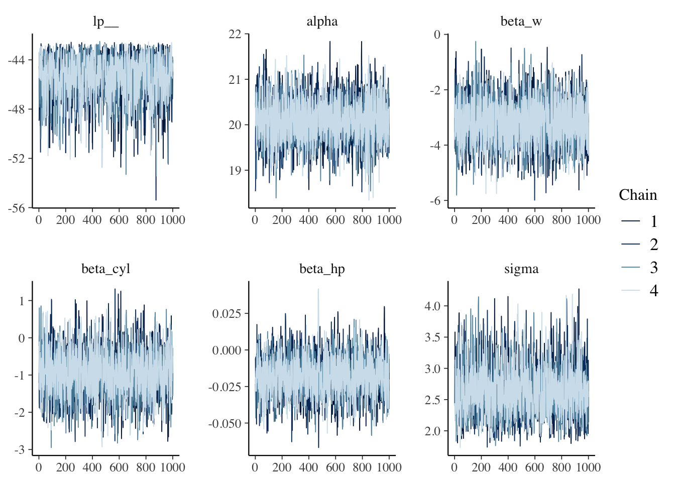
The fuzzy caterpillar appearance indicates that the chains are mixing well and have converged to a common distribution. We can also assess the Rhat values for each parameter. As a rule of thumb, Rhat values less than 1.05 indicate good convergence. The bayesplot package makes these calculations easy.
rhats <- rhat(linear.fit.3)
mcmc_rhat(rhats)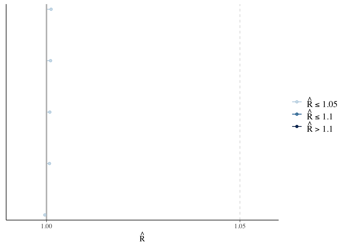
Effective Sample Size
The effective sample size estimates the number of independent draws from the posterior distribution of a given estimate. This metric is important because Markov chains can have autocorrelation which will lead to biased parameter estimates. With the bayesplot package we can visualize the ratio of the effective sample size to the total number of samples - the larger the ratio the better. The rule of thumb here is to worry about ratios less than 0.1.
eff.ratio <- neff_ratio(linear.fit.3)
eff.ratio
## alpha beta_w beta_cyl beta_hp sigma
## 0.8839743 0.8695231 0.6686701 0.7003035 0.6309044mcmc_neff(eff.ratio)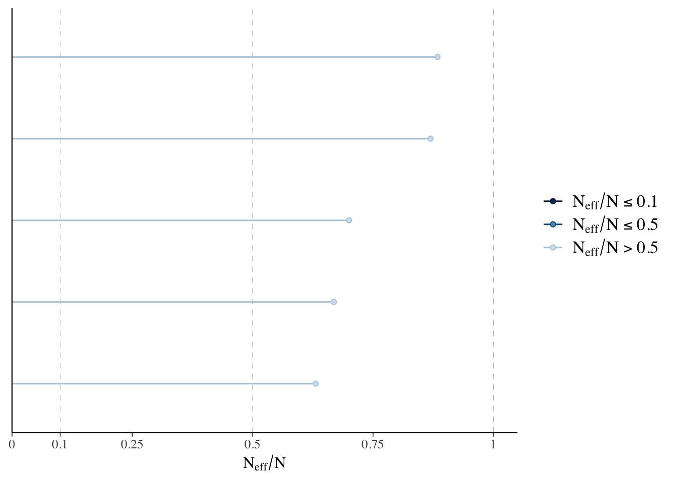
We can also check the autocorrelation in the chains with bayesplot. To use the mcmc_acf function, we’ll need to extract the posterior draws from the model.
mcmc_acf(fit.draws)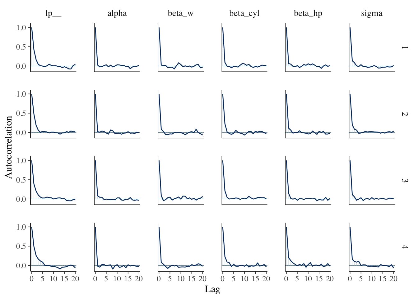
Here, we are looking to see how quickly the autocorrelation drops to zero.
Posterior Predictive Checks
One of the most powerful tools of Bayesian inference is to conduct posterior predictive checks. This check is designed to see how well our model can generate data that matches observed data. If we built a good model, it should be able to generate new observations that very closely resemble the observed data.
In order to perform posterior predictive checks, we will need to add in some code to our model. Specifically we need to calculate replications of our outcome variable. We can do this using the generated quantities section.
data {
  int n; //number of observations in the data
  vector[n] mpg; //vector of length n for the car's MPG
  vector[n] weight_c; //vector of length n for the car's weight
  vector[n] cylinders_c; ////vector of length n for the car's cylinders
  vector[n] hp_c; //vector of length n for the car's horsepower
}

parameters {
  real alpha; //the intercept parameter
  real beta_w; //slope parameter for weight
  real beta_cyl; //slope parameter for cylinder
  real beta_hp; //slope parameter for horsepower
  real<lower = 0> sigma; //variance parameter and restrict it to positive values
}

model {
  //linear predictor mu
  vector[n] mu;

  //write the linear equation
  mu = alpha + beta_w * weight_c + beta_cyl * cylinders_c + beta_hp * hp_c;

  //likelihood function
  mpg ~ normal(mu, sigma);
}

generated quantities {
  //replications for the posterior predictive distribution
  real y_rep[n] = normal_rng(alpha + beta_w * weight_c + beta_cyl *
    cylinders_c + beta_hp * hp_c, sigma);
}
In the code block above, normal_rng is the Stan function to generate observations from a normal distribution. So, y_rep generates new data points from a normal distribution using the linear model we built mu and a variance sigma. Now let’s re-estimate the model:
linear.fit.3 <- linear.model$sample(data = model.data, refresh = 0)## Running MCMC with 4 sequential chains...
##
## Chain 1 finished in 0.1 seconds.
## Chain 2 finished in 0.1 seconds.
## Chain 3 finished in 0.1 seconds.
## Chain 4 finished in 0.1 seconds.
##
## All 4 chains finished successfully.
## Mean chain execution time: 0.1 seconds.
## Total execution time: 0.9 seconds.print(linear.fit.3)## variable mean median sd mad q5 q95 rhat ess_bulk ess_tail
## lp__ -45.27 -44.93 1.77 1.62 -48.58 -43.13 1.01 1340 1990
## alpha 20.08 20.07 0.49 0.48 19.25 20.87 1.00 3018 2417
## beta_w -3.15 -3.16 0.77 0.76 -4.41 -1.88 1.00 2949 2618
## beta_cyl -0.95 -0.96 0.58 0.57 -1.89 0.00 1.00 2458 1928
## beta_hp -0.02 -0.02 0.01 0.01 -0.04 0.00 1.00 2763 2393
## sigma 2.64 2.60 0.38 0.36 2.10 3.33 1.00 2681 2335
## y_rep[1] 22.85 22.85 2.73 2.65 18.31 27.40 1.00 4020 4054
## y_rep[2] 21.97 22.02 2.74 2.72 17.50 26.46 1.00 3903 3851
## y_rep[3] 25.88 25.86 2.76 2.68 21.44 30.42 1.00 3879 3712
## y_rep[4] 20.89 20.92 2.74 2.65 16.31 25.28 1.00 3798 3738
##
## # showing 10 of 38 rows (change via 'max_rows' argument or 'cmdstanr_max_rows' option)In our model output, we now have a replicated y value for every row of data. We can use these values to plot the replicated data against the observed data.
y <- cars.data$mpg

# convert the cmdstanr fit to an rstan object
library(rstan)
## Loading required package: StanHeaders## rstan (Version 2.21.3, GitRev: 2e1f913d3ca3)## For execution on a local, multicore CPU with excess RAM we recommend calling
## options(mc.cores = parallel::detectCores()).
## To avoid recompilation of unchanged Stan programs, we recommend calling
## rstan_options(auto_write = TRUE)##
## Attaching package: 'rstan'## The following object is masked from 'package:tidyr':
##
## extractstanfit <- read_stan_csv(linear.fit.3$output_files())
# extract the fitted values
y.rep <- extract(stanfit)[["y_rep"]]
ppc_dens_overlay(y = cars.data$mpg, yrep = y.rep[1:100, ])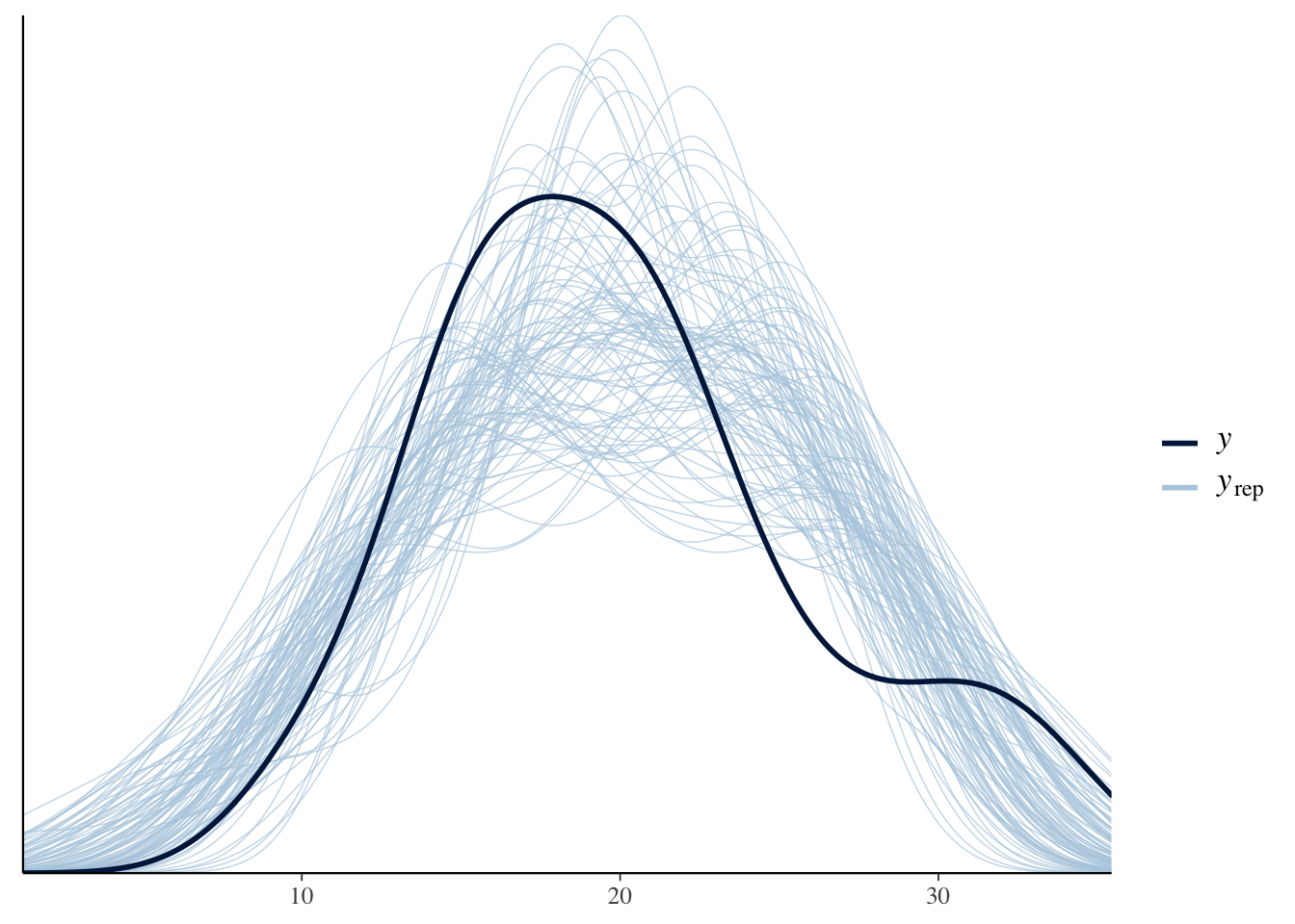
The closer the replicated values (yrep) get to the observed values (y) the more accurate the model. Here it looks like we could probably do a bit better, though the lose fit is likely due to the small sample size (which adds more uncertainty).
Improving the Model with Better Priors
To improve this model, let’s use more informative priors. Priors allow us to incorporate our background knowledge on the question into the model to produce more realistic estimates. For our question here, we probably don’t expect the weight of a vehicle to change its MPG more that a dozen or so miles per gallon. Unfortunately, because we didn’t specify priors in the previous models, it defaulted to using flat priors which essentially place an equal probably on all possible coefficient values - not very realistic. Let’s fix that.
To get a better sense of what priors to use, it’s a good idea to use prior predictive checks, which are a lot like posterior predictive checks only they don’t include any data. The goal is to select priors that put some probably over all plausible vales.
# expectations for the effect of weight on MPG
sample.weight <- rnorm(1000, mean = 0, sd = 100)
plot(density(sample.weight))
# expectations for the average mpg
sample.intercept <- rnorm(1000, mean = 0, sd = 100)
plot(density(sample.intercept))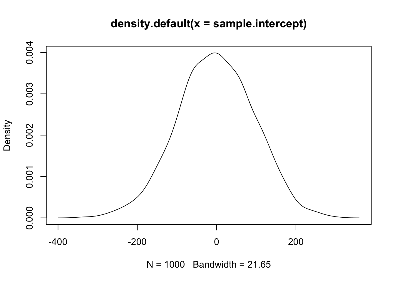
# expectations for model variance
sample.sigma <- runif(1000, min = 0, max = 100)
plot(density(sample.weight))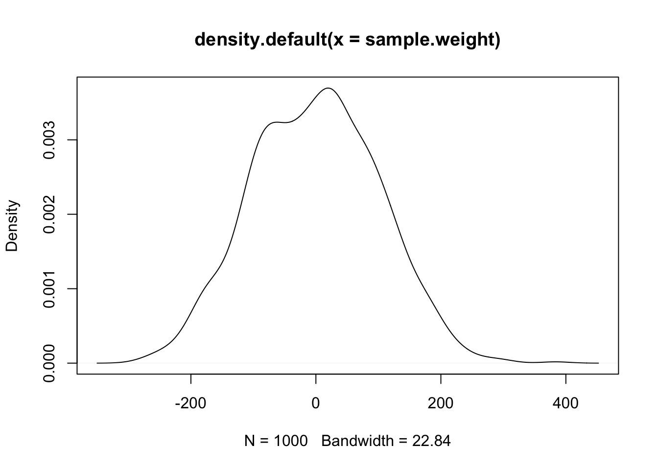
# prior predictive simulation for mpg given the priors
prior_mpg <- rnorm(1000, sample.weight + sample.intercept, sample.sigma)
plot(density(prior_mpg))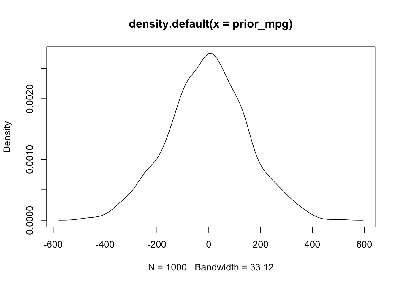
These priors suggest that the effect of weight on MPG could be anywhere from -400 to 400 points. Definitely not realistic - and these are already more informative priors than any frequentist analysis! Similarly, the expected MPG of a vehicle given these priors is anywhere from -400 to 400.
Let’s bring these in a bit.
# expectations for the effect of weight on MPG
sample.weight <- rnorm(1000, mean = -10, sd = 5)
plot(density(sample.weight))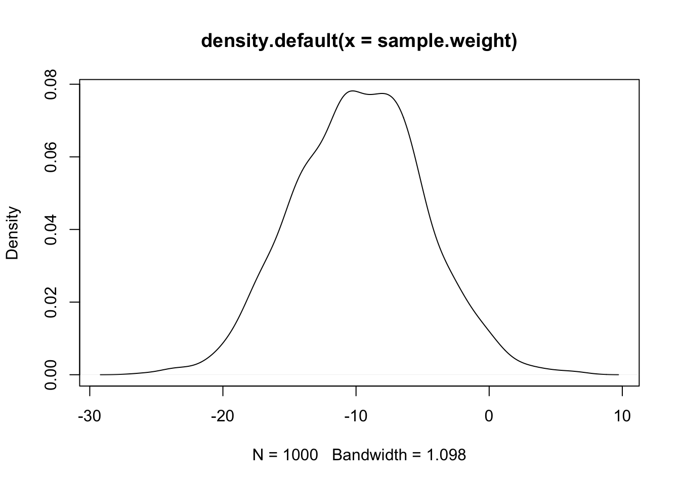
# expectations for the average mpg
sample.intercept <- rnorm(1000, mean = 20, sd = 5)
plot(density(sample.intercept))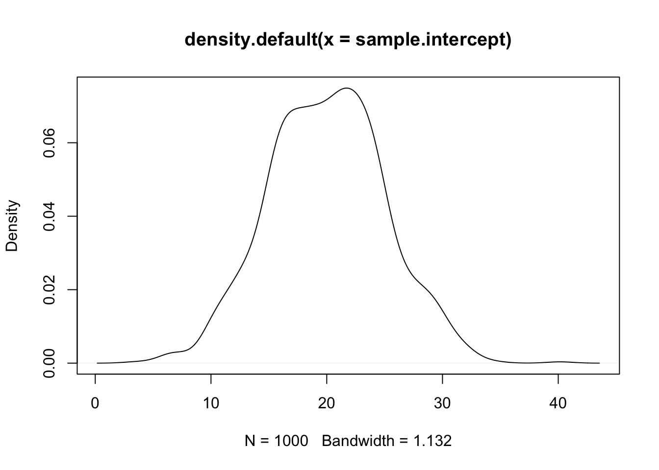
# expectations for model variance
sample.sigma <- runif(1000, min = 0, max = 10)
plot(density(sample.sigma))
# prior predictive simulation for mpg given the priors
prior_mpg <- rnorm(1000, sample.weight + sample.intercept, sample.sigma)
plot(density(prior_mpg))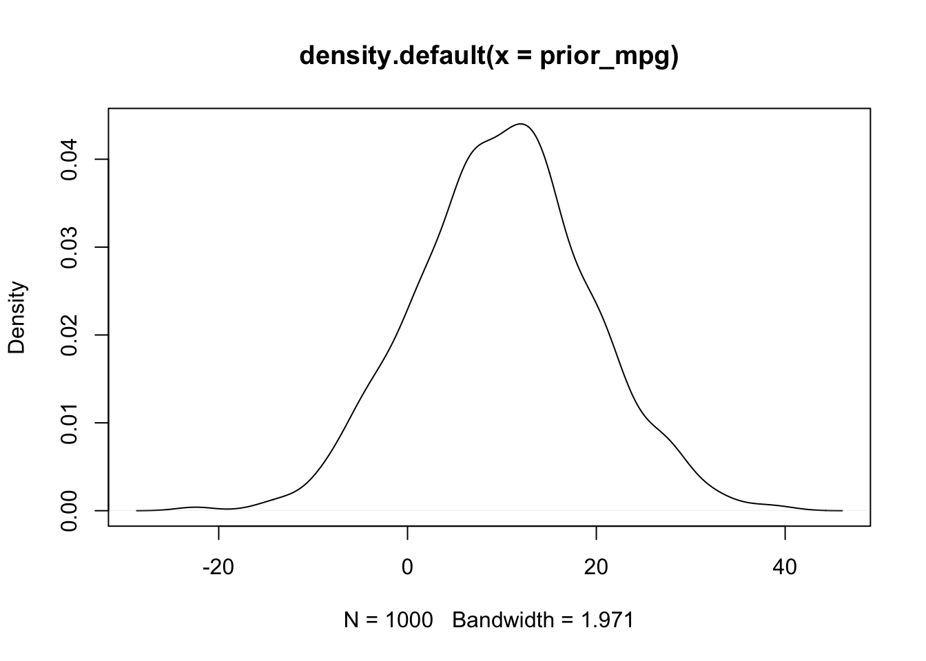
We could probably do better, but these look a lot better. Now the expected effect of weight on MPG is negative and and majority of the mass is concentrated between -15 and -5. Similarly, the expected MPG given these priors is between -10 and 20.
Now let’s build a new model with these priors and sample from it.
data {
  int n; //number of observations in the data
  vector[n] mpg; //vector of length n for the car's MPG
  vector[n] weight_c; //vector of length n for the car's weight
  vector[n] cylinders_c; ////vector of length n for the car's cylinders
  vector[n] hp_c; //vector of length n for the car's horsepower
}

parameters {
  real alpha; //the intercept parameter
  real beta_w; //slope parameter for weight
  real beta_cyl; //slope parameter for cylinder
  real beta_hp; //slope parameter for horsepower
  real<lower = 0> sigma; //variance parameter and restrict it to positive values
}

model {
  //linear predictor mu
  vector[n] mu;

  //write the linear equation
  mu = alpha + beta_w * weight_c + beta_cyl * cylinders_c + beta_hp * hp_c;

  //prior expectations
  alpha ~ normal(20, 5);
  beta_w ~ normal(-10, 5);
  beta_cyl ~ normal(0, 5); //we'll include my uncertain priors here
  beta_hp ~ normal(0, 5); //we'll include my uncertain priors here
  sigma ~ uniform(0, 10);

  //likelihood function
  mpg ~ normal(mu, sigma);
}

generated quantities {
  //replications for the posterior predictive distribution
  real y_rep[n] = normal_rng(alpha + beta_w * weight_c + beta_cyl *
  cylinders_c + beta_hp * hp_c, sigma);
}
Now sample:
linear.fit.4 <- linear.model$sample(data = model.data)## Running MCMC with 4 sequential chains...
##
## Chain 1 Iteration: 1 / 2000 [ 0%] (Warmup)
## Chain 1 Iteration: 100 / 2000 [ 5%] (Warmup)
## Chain 1 Iteration: 200 / 2000 [ 10%] (Warmup)
## Chain 1 Iteration: 300 / 2000 [ 15%] (Warmup)
## Chain 1 Iteration: 400 / 2000 [ 20%] (Warmup)
## Chain 1 Iteration: 500 / 2000 [ 25%] (Warmup)
## Chain 1 Iteration: 600 / 2000 [ 30%] (Warmup)
## Chain 1 Iteration: 700 / 2000 [ 35%] (Warmup)
## Chain 1 Iteration: 800 / 2000 [ 40%] (Warmup)
## Chain 1 Iteration: 900 / 2000 [ 45%] (Warmup)
## Chain 1 Iteration: 1000 / 2000 [ 50%] (Warmup)
## Chain 1 Iteration: 1001 / 2000 [ 50%] (Sampling)
## Chain 1 Iteration: 1100 / 2000 [ 55%] (Sampling)
## Chain 1 Iteration: 1200 / 2000 [ 60%] (Sampling)
## Chain 1 Iteration: 1300 / 2000 [ 65%] (Sampling)
## Chain 1 Iteration: 1400 / 2000 [ 70%] (Sampling)
## Chain 1 Iteration: 1500 / 2000 [ 75%] (Sampling)
## Chain 1 Iteration: 1600 / 2000 [ 80%] (Sampling)
## Chain 1 Iteration: 1700 / 2000 [ 85%] (Sampling)
## Chain 1 Iteration: 1800 / 2000 [ 90%] (Sampling)
## Chain 1 Iteration: 1900 / 2000 [ 95%] (Sampling)
## Chain 1 Iteration: 2000 / 2000 [100%] (Sampling)
## Chain 1 finished in 0.1 seconds.
## Chain 2 Iteration: 1 / 2000 [ 0%] (Warmup)
## Chain 2 Iteration: 100 / 2000 [ 5%] (Warmup)
## Chain 2 Iteration: 200 / 2000 [ 10%] (Warmup)
## Chain 2 Iteration: 300 / 2000 [ 15%] (Warmup)
## Chain 2 Iteration: 400 / 2000 [ 20%] (Warmup)
## Chain 2 Iteration: 500 / 2000 [ 25%] (Warmup)
## Chain 2 Iteration: 600 / 2000 [ 30%] (Warmup)
## Chain 2 Iteration: 700 / 2000 [ 35%] (Warmup)
## Chain 2 Iteration: 800 / 2000 [ 40%] (Warmup)
## Chain 2 Iteration: 900 / 2000 [ 45%] (Warmup)
## Chain 2 Iteration: 1000 / 2000 [ 50%] (Warmup)
## Chain 2 Iteration: 1001 / 2000 [ 50%] (Sampling)
## Chain 2 Iteration: 1100 / 2000 [ 55%] (Sampling)
## Chain 2 Iteration: 1200 / 2000 [ 60%] (Sampling)
## Chain 2 Iteration: 1300 / 2000 [ 65%] (Sampling)
## Chain 2 Iteration: 1400 / 2000 [ 70%] (Sampling)
## Chain 2 Iteration: 1500 / 2000 [ 75%] (Sampling)
## Chain 2 Iteration: 1600 / 2000 [ 80%] (Sampling)
## Chain 2 Iteration: 1700 / 2000 [ 85%] (Sampling)
## Chain 2 Iteration: 1800 / 2000 [ 90%] (Sampling)
## Chain 2 Iteration: 1900 / 2000 [ 95%] (Sampling)
## Chain 2 Iteration: 2000 / 2000 [100%] (Sampling)
## Chain 2 finished in 0.2 seconds.
## Chain 3 Iteration: 1 / 2000 [ 0%] (Warmup)
## Chain 3 Iteration: 100 / 2000 [ 5%] (Warmup)
## Chain 3 Iteration: 200 / 2000 [ 10%] (Warmup)
## Chain 3 Iteration: 300 / 2000 [ 15%] (Warmup)
## Chain 3 Iteration: 400 / 2000 [ 20%] (Warmup)
## Chain 3 Iteration: 500 / 2000 [ 25%] (Warmup)
## Chain 3 Iteration: 600 / 2000 [ 30%] (Warmup)
## Chain 3 Iteration: 700 / 2000 [ 35%] (Warmup)
## Chain 3 Iteration: 800 / 2000 [ 40%] (Warmup)
## Chain 3 Iteration: 900 / 2000 [ 45%] (Warmup)
## Chain 3 Iteration: 1000 / 2000 [ 50%] (Warmup)
## Chain 3 Iteration: 1001 / 2000 [ 50%] (Sampling)
## Chain 3 Iteration: 1100 / 2000 [ 55%] (Sampling)
## Chain 3 Iteration: 1200 / 2000 [ 60%] (Sampling)
## Chain 3 Iteration: 1300 / 2000 [ 65%] (Sampling)
## Chain 3 Iteration: 1400 / 2000 [ 70%] (Sampling)
## Chain 3 Iteration: 1500 / 2000 [ 75%] (Sampling)
## Chain 3 Iteration: 1600 / 2000 [ 80%] (Sampling)
## Chain 3 Iteration: 1700 / 2000 [ 85%] (Sampling)
## Chain 3 Iteration: 1800 / 2000 [ 90%] (Sampling)
## Chain 3 Iteration: 1900 / 2000 [ 95%] (Sampling)
## Chain 3 Iteration: 2000 / 2000 [100%] (Sampling)
## Chain 3 finished in 0.2 seconds.
## Chain 4 Iteration: 1 / 2000 [ 0%] (Warmup)
## Chain 4 Iteration: 100 / 2000 [ 5%] (Warmup)
## Chain 4 Iteration: 200 / 2000 [ 10%] (Warmup)
## Chain 4 Iteration: 300 / 2000 [ 15%] (Warmup)
## Chain 4 Iteration: 400 / 2000 [ 20%] (Warmup)
## Chain 4 Iteration: 500 / 2000 [ 25%] (Warmup)
## Chain 4 Iteration: 600 / 2000 [ 30%] (Warmup)
## Chain 4 Iteration: 700 / 2000 [ 35%] (Warmup)
## Chain 4 Iteration: 800 / 2000 [ 40%] (Warmup)
## Chain 4 Iteration: 900 / 2000 [ 45%] (Warmup)
## Chain 4 Iteration: 1000 / 2000 [ 50%] (Warmup)
## Chain 4 Iteration: 1001 / 2000 [ 50%] (Sampling)
## Chain 4 Iteration: 1100 / 2000 [ 55%] (Sampling)
## Chain 4 Iteration: 1200 / 2000 [ 60%] (Sampling)
## Chain 4 Iteration: 1300 / 2000 [ 65%] (Sampling)
## Chain 4 Iteration: 1400 / 2000 [ 70%] (Sampling)
## Chain 4 Iteration: 1500 / 2000 [ 75%] (Sampling)
## Chain 4 Iteration: 1600 / 2000 [ 80%] (Sampling)
## Chain 4 Iteration: 1700 / 2000 [ 85%] (Sampling)
## Chain 4 Iteration: 1800 / 2000 [ 90%] (Sampling)
## Chain 4 Iteration: 1900 / 2000 [ 95%] (Sampling)
## Chain 4 Iteration: 2000 / 2000 [100%] (Sampling)
## Chain 4 finished in 0.2 seconds.
##
## All 4 chains finished successfully.
## Mean chain execution time: 0.2 seconds.
## Total execution time: 1.0 seconds.print(linear.fit.4)## variable mean median sd mad q5 q95 rhat ess_bulk ess_tail
## lp__ -48.56 -45.78 13.93 1.58 -51.03 -44.03 1.02 167 27
## alpha 19.58 20.09 2.90 0.47 19.08 20.86 1.03 154 27
## beta_w -3.28 -3.33 0.92 0.74 -4.59 -2.00 1.01 476 116
## beta_cyl -0.89 -0.88 0.67 0.59 -1.90 0.11 1.01 619 137
## beta_hp -0.02 -0.02 0.01 0.01 -0.04 0.00 1.01 2127 1639
## sigma 2.86 2.59 1.33 0.35 2.11 3.52 1.02 134 29
## y_rep[1] 22.38 22.80 4.47 2.89 17.37 27.32 1.02 194 42
## y_rep[2] 21.52 21.98 4.40 2.71 16.69 26.51 1.02 160 36
## y_rep[3] 25.43 25.82 4.21 2.86 20.33 30.44 1.02 227 42
## y_rep[4] 20.42 20.92 4.38 2.81 15.20 25.37 1.02 236 40
##
## # showing 10 of 38 rows (change via 'max_rows' argument or 'cmdstanr_max_rows' option)After estimating the model with more informative priors, the lp__ is now a little bit lower. We can compare the prior distribution to the posterior distribution to see how “powerful” our priors are.
linear.fit.4 <- read_stan_csv(linear.fit.4$output_files())
posterior <- as.data.frame(linear.fit.4)

library(tidyverse)
ggplot() +
  geom_density(aes(x = sample.weight)) +
  geom_density(aes(x = posterior$beta_w), color = "blue")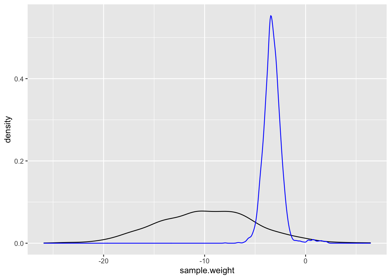
Here we can see that even with more “informative priors” they are still very weak compared to the data.
Summarize the Model
With our final model in hand, we can visualizations of our model’s results.
Coeficient Plot
stan_plot(linear.fit.4,
          pars = c("alpha", "beta_w", "beta_cyl", "beta_hp", "sigma"))
## ci_level: 0.8 (80% intervals)## outer_level: 0.95 (95% intervals)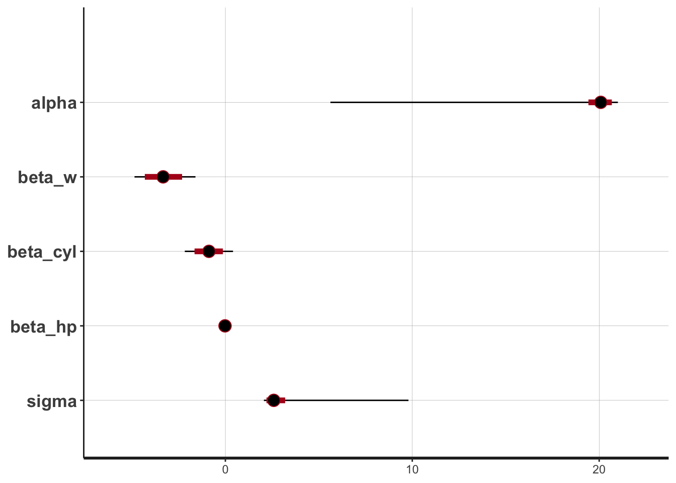
Fitted Regression Line
Here we can plot the fitted regression line
# Fitted Line
ggplot(data = cars.data, aes(x = weight_c, y = mpg)) +
  geom_point() +
  stat_function(fun = function(x) mean(posterior$alpha) + mean(posterior$beta_w) * x)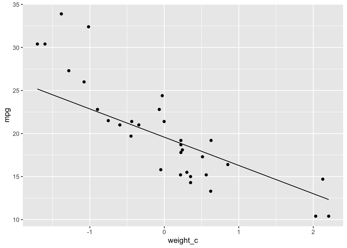
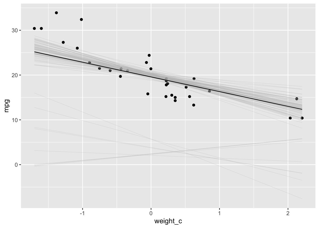
# Fitted Line with Uncertainty ------------------------------------------------
fit.plot <-
  ggplot(data = cars.data, aes(x = weight_c, y = mpg)) +
  geom_point()

# select a random sample of 100 draws from the posterior distribution
sims <-
  posterior %>%
  mutate(n = row_number()) %>%
  sample_n(size = 100)

# add these draws to the plot
lines <-
  purrr::map(1:100, function(i) stat_function(fun = function(x) sims[i, 1] + sims[i, 2] * x,
             size = 0.08, color = "gray"))
fit.plot <- fit.plot + lines

# add the mean line to the plot
fit.plot <-
  fit.plot +
  stat_function(fun = function(x) mean(posterior$alpha) + mean(posterior$beta_w) * x)

fit.plot