Logit and Probit Models
In the last tutorial, we learned how to program and estimate linear models in Stan. In this tutorial, we’ll learn how to estimate binary outcome models commonly referred to as Logit and Probit.
Let’s get right into it.
Logit with the Bernoulli Distribution
Import Data
This time, we’ll use a data on graduate school applicants. This data includes each applicant’s GRE score, GPA, the rank of their undergraduate school, and whether or not they were admitted to graduate school. Our goal is to predict the probability that a student will be admitted.
gre.data <- read.csv("https://stats.idre.ucla.edu/stat/data/binary.csv")

library(tidyverse)
glimpse(gre.data)
## Rows: 400
## Columns: 4
## $ admit <int> 0, 1, 1, 1, 0, 1, 1, 0, 1, 0, 0, 0, 1, 0, 1, 0, 0, 0, 0, 1, 0, 1…
## $ gre <int> 380, 660, 800, 640, 520, 760, 560, 400, 540, 700, 800, 440, 760,…
## $ gpa <dbl> 3.61, 3.67, 4.00, 3.19, 2.93, 3.00, 2.98, 3.08, 3.39, 3.92, 4.00…
## $ rank <int> 3, 3, 1, 4, 4, 2, 1, 2, 3, 2, 4, 1, 1, 2, 1, 3, 4, 3, 2, 1, 3, 2…We could predict whether or not a student is admitted with a Gaussian likelihood function, but then we would be assuming that the outcome is continuous and that both positive and negative values are possible. These are bad assumptions. This data is generated by a process that only produces positive and discrete outcomes. Each application either results in an admit or a reject, values in between are impossible. This means that we’ll need to use a different likelihood function. The Bernoulli distribution seems like a good fit.
The Bernoulli distribution is a probability distribution for a random variable that can have an outcome of 1 with probability \(p\) and an outcome of 0 with a probability of \(q = 1 - p\). A quick look at the distribution shows that it produces values of 0 and 1.
plot(rbernoulli(100, p = 0.5))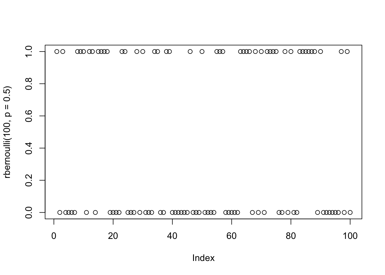
You’re probably used to using a binomial likelihood for Logit and Probit models, but the binomial distribution is really meant to describe aggregated counts. The binomial distribution includes an additional parameter for the number of trials that occurred. We’ll see an example of this later. The Bernoulli distribution is essentially equivalent to a binomial distribution with only 1 trial.
Build a Logit Model
Here is the model that we want to estimate in Stan:
\[ \begin{aligned} \text{admit} &\sim \text{Bernoulli}(p) \\ \text{Logit}(p) &= \alpha + \beta_1 \text{GRE Score} + \beta_2 \text{GPA} + \beta_3 \text{Undergrad Ranking} \end{aligned} \]
Here we are interesting in estimating the probability that a given student is admitted \(p\) using their GRE score, their GPA, and the ranking of their undergraduate school. Notice that we have an additional function in this model: the Logit() function.
This function is known as a “link” function because it maps the observed 0-1 outcome onto the range of 0-1.0. This link function will prevent the model from predicting outcomes above 1.0 or below 0. When we built our linear model with the normal distribution in the last tutorial, we didn’t need a link function because we were estimating the mean of a continuous outcome (technically we used the identity link function).
Let’s load CmdStanR,
library(cmdstanr)## This is cmdstanr version 0.4.0## - Online documentation and vignettes at mc-stan.org/cmdstanr## - CmdStan path set to: /Users/nickjenkins/.cmdstanr/cmdstan-2.28.1## - Use set_cmdstan_path() to change the path##
## A newer version of CmdStan is available. See ?install_cmdstan() to install it.
## To disable this check set option or environment variable CMDSTANR_NO_VER_CHECK=TRUE.register_knitr_engine(override = FALSE) # This registers cmdstanr with knitr so that we can use
# it with R Markdown.then program the model:
data {
  int n; //number of observations in the data
  int<lower = 0, upper = 1> admit[n]; //integer of length n for admission decision
  vector[n] gre; //vector of length n for GRE scores
  vector[n] gpa; //vector of length n for GPA
  vector[n] ranking; //vector of length n for school ranking
}

parameters {
  real alpha; //intercept parameter
  vector[3] beta; //vector of coefficients
}

model {
  //linear predictor
  vector[n] p;

  //linear equation
  p = alpha + beta[1] * gre + beta[2] * gpa + beta[3] * ranking;

  //likelihood and link function
  admit ~ bernoulli_logit(p);
}
Now let’s prepare the data and estimate the model.
library(tidybayes)

model.data <-
  gre.data %>%
  rename(ranking = rank) %>%
  compose_data()

# sample
logit.fit <- logit.model$sample(data = model.data, refresh = 0)
## Running MCMC with 4 sequential chains...
##
## Chain 1 finished in 4.2 seconds.
## Chain 2 finished in 4.2 seconds.
## Chain 3 finished in 4.3 seconds.
## Chain 4 finished in 4.2 seconds.
##
## All 4 chains finished successfully.
## Mean chain execution time: 4.2 seconds.
## Total execution time: 17.3 seconds.# print results
print(logit.fit)## variable mean median sd mad q5 q95 rhat ess_bulk ess_tail
## lp__ -231.69 -231.35 1.42 1.16 -234.50 -230.05 1.00 1474 1956
## alpha -3.52 -3.52 1.12 1.14 -5.36 -1.73 1.00 1312 1607
## beta[1] 0.00 0.00 0.00 0.00 0.00 0.00 1.00 3190 2345
## beta[2] 0.79 0.80 0.33 0.33 0.26 1.33 1.00 1507 1491
## beta[3] -0.57 -0.57 0.12 0.12 -0.77 -0.37 1.00 1746 1925Here are the interpretations of each coefficient. Notice that they are a bit different since we are using a Logit link function. We can “undo” the link function to convert each estimate back to the linear scale.
alpha: For a student with a 0 on the GRE, a GPA of 0, and an undergraduate school ranking of 0, the expected admission probability is \(logit^{-1}(-3.51)\), which we can calculate in R withplogis(-3.51)* 100 = 2.9029036 percent.beta[1]: Comparing two applicants who differ by 1 point on the GRE, the model predicts a positive difference in the probability of admission of about 50%.beta[2]: Comparing two applicants who differ by 1 point in their GPA, the model predicts a positive difference in the probability of admission of about 68%.beta[3]: Comparing two applicants who differ by 1 point in their undergrad school ranking, the model predicts a positive difference in the probability of admission of about 0.36%.
When dealing with the logit models, plots can go a long way towards helping us understand the results. We’ll plot the relationship between admission and GPA.
library(rstan)## Loading required package: StanHeaders## rstan (Version 2.21.3, GitRev: 2e1f913d3ca3)## For execution on a local, multicore CPU with excess RAM we recommend calling
## options(mc.cores = parallel::detectCores()).
## To avoid recompilation of unchanged Stan programs, we recommend calling
## rstan_options(auto_write = TRUE)##
## Attaching package: 'rstan'## The following object is masked from 'package:tidyr':
##
## extractlogit.fit <- read_stan_csv(logit.fit$output_files())
logit.coefs <-
as.data.frame(logit.fit, pars = c("alpha", "beta[1]", "beta[2]", "beta[3]")) %>%
summarise(alpha = mean(alpha),
beta_1 = mean(`beta[1]`),
beta_2 = mean(`beta[2]`),
beta_3 = mean(`beta[3]`))
ggplot(data = gre.data, aes(x = gpa, y = admit)) +
geom_point(position = position_jitter(width = 0, height = 0.05), shape = 1) +
stat_function(fun = function(x) plogis(logit.coefs$alpha + logit.coefs$beta_2 * x))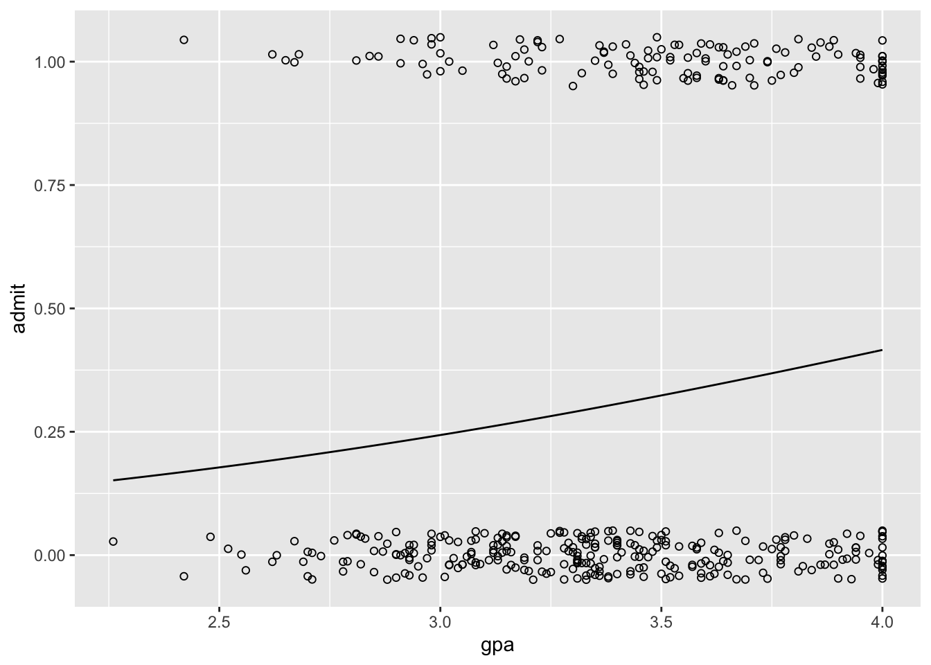
# sims <- as.data.frame(logit.fit)
# sims <-
#   sims %>%
#   mutate(n = row_number()) %>%
#   sample_n(size = 100)
#
# lines <- purrr::map(1:100, function(i) stat_function(fun = function(x) invlogit(sims[i, 1] + sims[i, 4] * x),
#                                                      size = 0.08, color = "gray"))
# success.plot <- success.plot + lines
# success.plot <-
#   success.plot +
#   stat_function(fun = function(x) invlogit(fixef(logit.fit)[1] + fixef(logit.fit)[4] * x),
#                 size = 1)
# success.plot
We can also add uncertainty to the plot:
plot <-
  ggplot(data = gre.data, aes(x = gpa, y = admit)) +
  geom_point(position = position_jitter(width = 0, height = 0.05), shape = 1)

sims <- as.data.frame(logit.fit)
sims <-
  sims %>%
  mutate(n = row_number()) %>%
  sample_n(size = 100) # select a random sample of 100 values from the posterior

lines <-
  purrr::map(1:100, function(i) stat_function(fun = function(x) plogis(sims[i, 1] + sims[i, 3] * x),
                                              size = 0.1, color = "gray"))

plot <- plot + lines
plot <-
  plot + stat_function(fun = function(x) plogis(logit.coefs$alpha + logit.coefs$beta_2 * x))
plot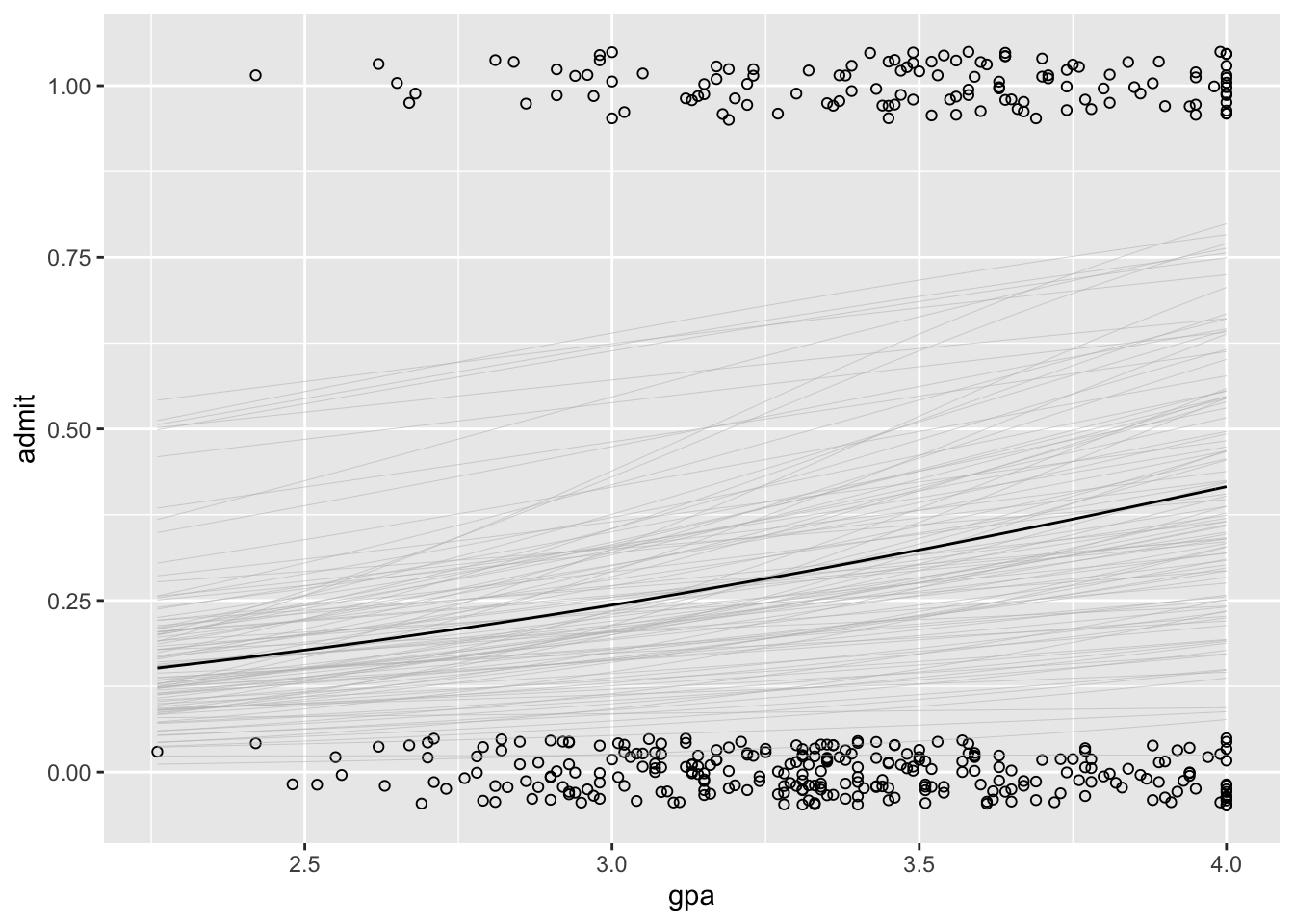
Picking Priors for Logit Models
When we are thinking about priors for logit models (or any generalized linear model), it’s important to use the inverse link function to convert back to the linear scale. With the Gaussian model, we can just plot our priors “as-is”, but with logit models we need to “undue” the link function. What is a weak prior on the linear scale might be really informative on the logit scale. To illustrate just how different priors can be, let’s start by using standard weakly informative priors for a normal distribution.
# expectations for the average admission rate
sample.intercept <- rnorm(1000, mean = 0, sd = 10)
plot(density(plogis(sample.intercept)))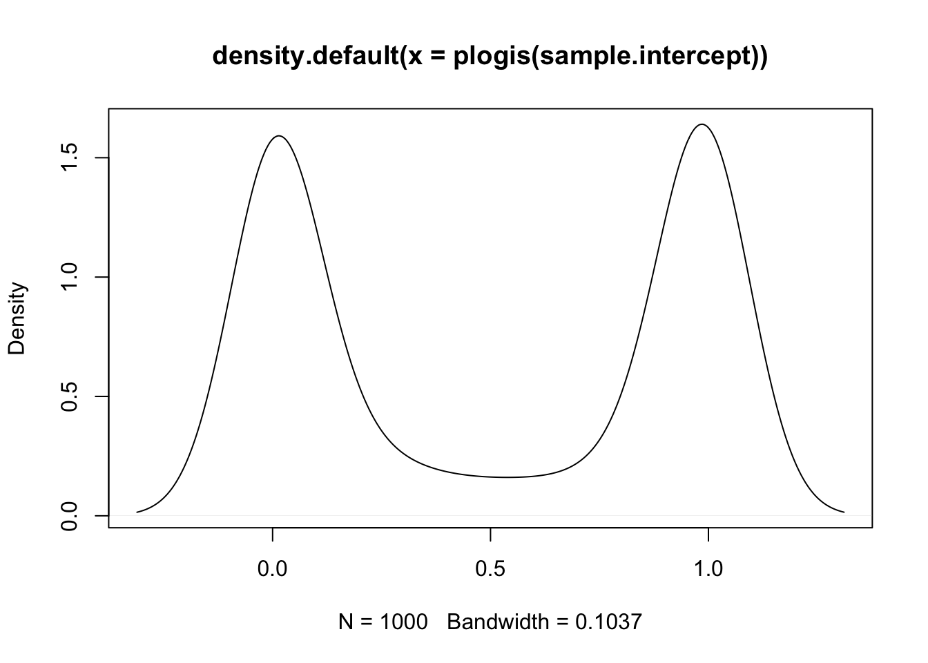
With this prior, the model thinks that applicants are either never get accepted or that they always get accepted. This is extreme and we can do better:
sample.intercept <- rnorm(1000, mean = 0, sd = 1.5)
plot(density(plogis(sample.intercept)))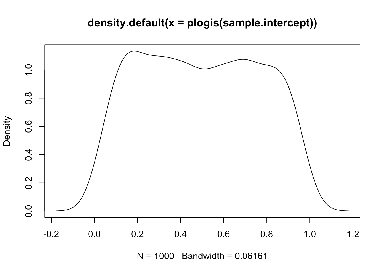
This is still wide, but already a lot more reasonable. Let’s simulate the rest of the priors.
# expectations for the average admission rate (around 26%)
sample.intercept <- rnorm(1000, mean = -1, sd = 1.5)
plot(density(plogis(sample.intercept)))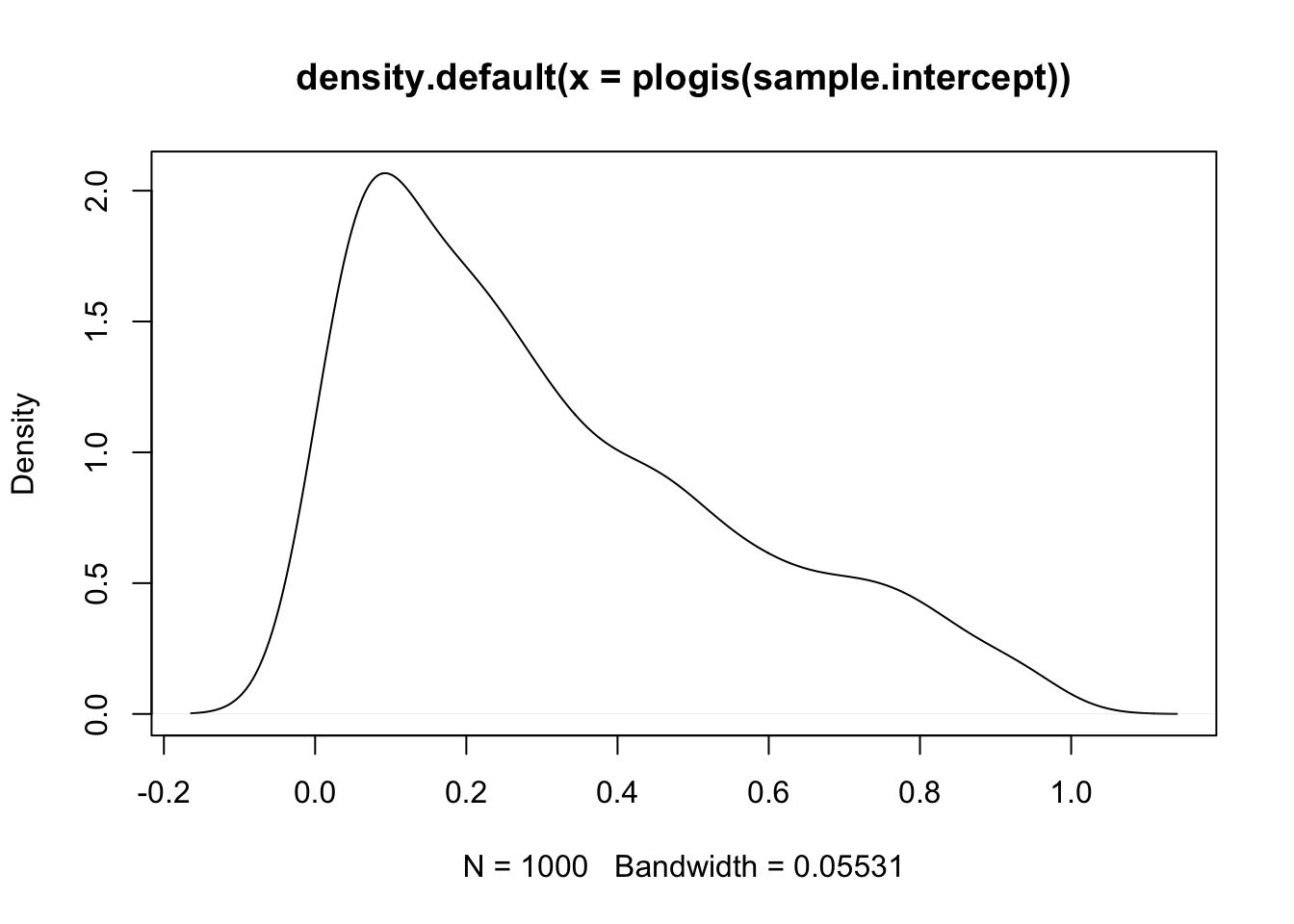
# expectations for the effect of GRE on admission
sample.gre <- rnorm(1000, mean = 0.5, sd = 1)
plot(density(plogis(sample.gre)))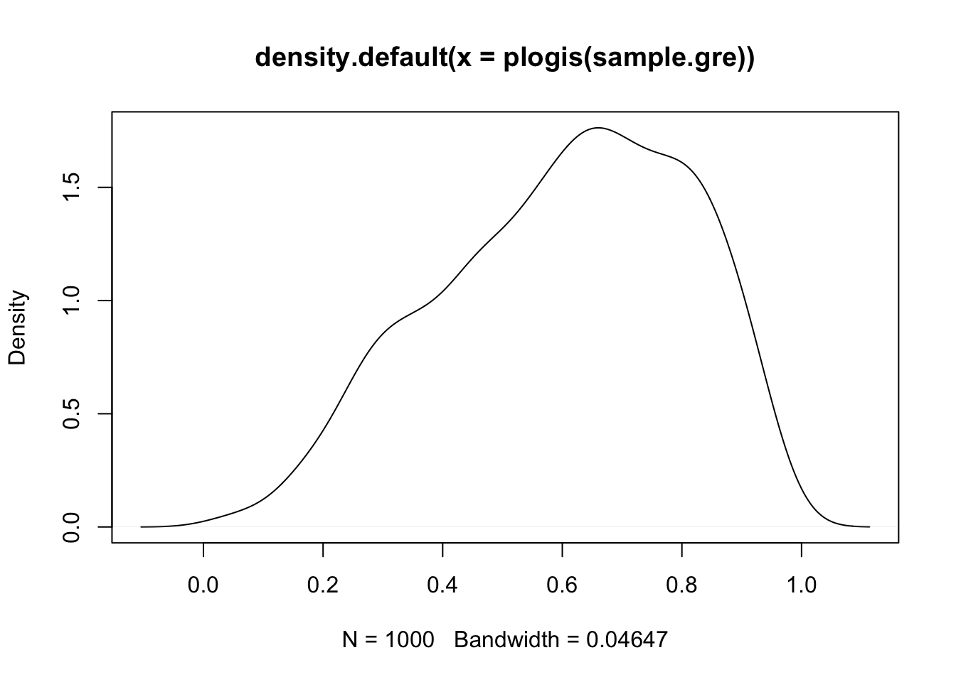
# prior predictive simulation for admission given the priors
prior_admit <- rbernoulli(1000, plogis(sample.gre + sample.intercept))
plot(density(as.numeric(prior_admit)))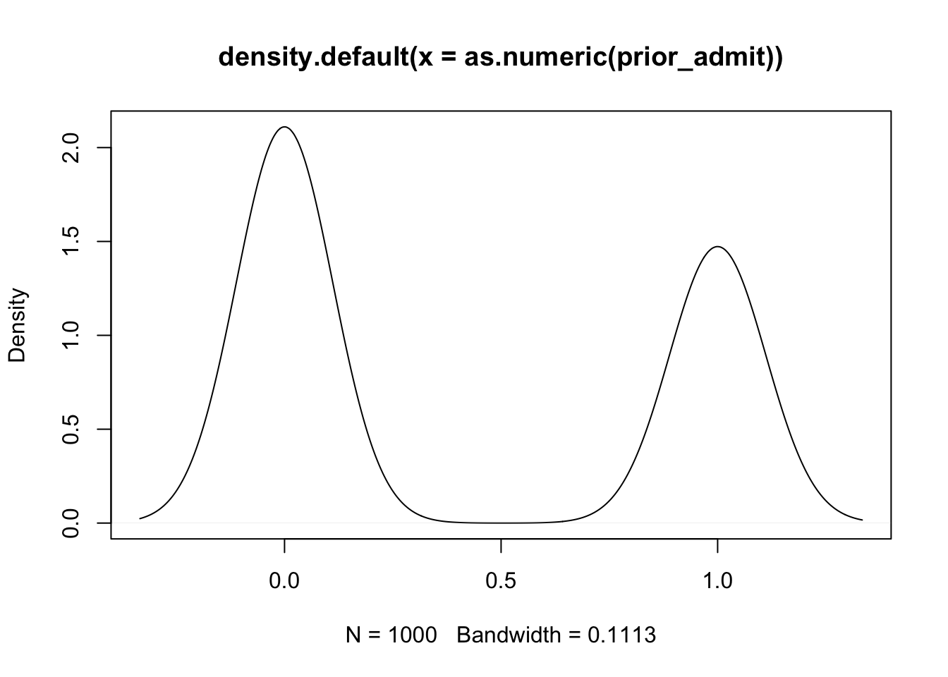
Here the model expects that more people are rejected than are accepted. Now we can add these priors into the model:
data {
  int n; //number of observations in the data
  int<lower = 0, upper = 1> admit[n]; //integer of length n for admission decision
  vector[n] gre; //vector of length n for GRE scores
  vector[n] gpa; //vector of length n for GPA
  vector[n] ranking; //vector of length n for school ranking
}

parameters {
  real alpha; //intercept parameter
  vector[3] beta; //vector of coefficients
}

model {
  //linear predictor
  vector[n] p;

  //linear equation
  p = alpha + beta[1] * gre + beta[2] * gpa + beta[3] * ranking;

  //prior expectations
  alpha ~ normal(-1, 1.5);
  beta ~ normal(0.5, 1.0);

  //likelihood and link function
  admit ~ bernoulli_logit(p);
}
and restimate the model:
# sample
logit.fit <- logit.model$sample(data = model.data, refresh = 0)
## Running MCMC with 4 sequential chains...
##
## Chain 1 finished in 4.4 seconds.
## Chain 2 finished in 4.5 seconds.
## Chain 3 finished in 4.2 seconds.
## Chain 4 finished in 3.9 seconds.
##
## All 4 chains finished successfully.
## Mean chain execution time: 4.2 seconds.
## Total execution time: 17.3 seconds.# print results
print(logit.fit)## variable mean median sd mad q5 q95 rhat ess_bulk ess_tail
## lp__ -233.29 -232.99 1.37 1.21 -235.91 -231.66 1.00 1620 2355
## alpha -2.61 -2.61 0.86 0.88 -4.03 -1.23 1.00 1342 1842
## beta[1] 0.00 0.00 0.00 0.00 0.00 0.00 1.00 2825 2334
## beta[2] 0.57 0.58 0.27 0.27 0.12 1.02 1.00 1556 2109
## beta[3] -0.58 -0.57 0.12 0.12 -0.78 -0.37 1.00 1630 1940Finally, we can add in posterior predictive draws in the generated quantities block like this:
data {
  int n; //number of observations in the data
  int<lower = 0, upper = 1> admit[n]; //integer of length n for admission decision
  vector[n] gre; //vector of length n for GRE scores
  vector[n] gpa; //vector of length n for GPA
  vector[n] ranking; //vector of length n for school ranking
}

parameters {
  real alpha; //intercept parameter
  vector[3] beta; //vector of coefficients
}

model {
  //linear predictor
  vector[n] p;

  //linear equation
  p = alpha + beta[1] * gre + beta[2] * gpa + beta[3] * ranking;

  //prior expectations
  alpha ~ normal(-1, 1.5);
  beta ~ normal(0.5, 1.0);

  //likelihood and link function
  admit ~ bernoulli_logit(p);
}

generated quantities {
  //replications for the posterior predictive distribution
  real y_rep[n] = bernoulli_logit_rng(alpha + beta[1] * gre + beta[2] * gpa +
    beta[3] * ranking);
}
logit.fit <- logit.model$sample(data = model.data, refresh = 0)## Running MCMC with 4 sequential chains...
##
## Chain 1 finished in 4.2 seconds.
## Chain 2 finished in 4.7 seconds.
## Chain 3 finished in 4.5 seconds.
## Chain 4 finished in 4.2 seconds.
##
## All 4 chains finished successfully.
## Mean chain execution time: 4.4 seconds.
## Total execution time: 18.0 seconds.print(logit.fit)## variable mean median sd mad q5 q95 rhat ess_bulk ess_tail
## lp__ -233.25 -232.91 1.43 1.23 -236.13 -231.62 1.00 1419 1971
## alpha -2.64 -2.65 0.88 0.87 -4.11 -1.22 1.00 1504 1793
## beta[1] 0.00 0.00 0.00 0.00 0.00 0.00 1.00 3066 2299
## beta[2] 0.58 0.58 0.27 0.27 0.15 1.02 1.00 1576 2083
## beta[3] -0.58 -0.58 0.12 0.12 -0.78 -0.37 1.00 1608 1567
## y_rep[1] 0.20 0.00 0.40 0.00 0.00 1.00 1.00 4052 NA
## y_rep[2] 0.31 0.00 0.46 0.00 0.00 1.00 1.00 3954 NA
## y_rep[3] 0.70 1.00 0.46 0.00 0.00 1.00 1.00 3926 NA
## y_rep[4] 0.16 0.00 0.37 0.00 0.00 1.00 1.00 4085 NA
## y_rep[5] 0.10 0.00 0.31 0.00 0.00 1.00 1.00 3910 NA
##
## # showing 10 of 405 rows (change via 'max_rows' argument or 'cmdstanr_max_rows' option)stanfit <- read_stan_csv(logit.fit$output_files())
# extract the fitted values
y.rep <- rstan::extract(stanfit)[["y_rep"]]
y <- gre.data$admit
library(bayesplot)
ppc_ecdf_overlay(y, y.rep[sample(nrow(y.rep), 100), ], discrete = TRUE)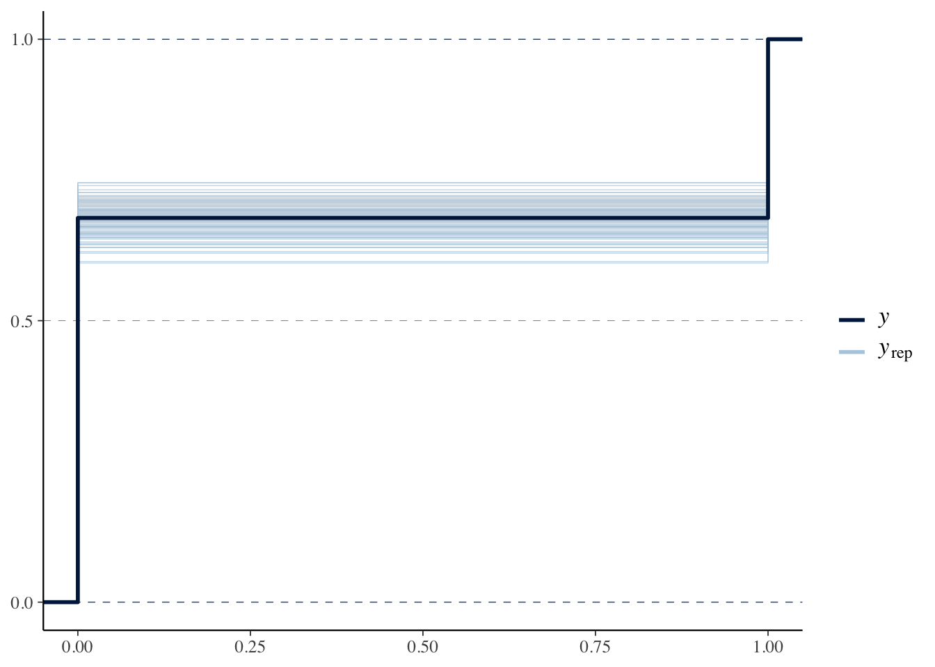
Probit Model with the Bernoulli Distribution
We can change the logit link to a probit link with the Phi function in Stan, which is the cumulative normal distribution function:
data {
  int n; //number of observations in the data
  int<lower = 0, upper = 1> admit[n]; //integer of length n for admission decision
  vector[n] gre; //vector of length n for GRE scores
  vector[n] gpa; //vector of length n for GPA
  vector[n] ranking; //vector of length n for school ranking
}

parameters {
  real alpha; //intercept parameter
  vector[3] beta; //vector of coefficients
}

model {
  //linear model
  vector[n] p;
  p = alpha + beta[1] * gre + beta[2] * gpa + beta[3] * ranking;

  //likelihood and link function
  admit ~ bernoulli(Phi(p));
}
We already have the data ready, so we can get right to sampling from the model.
probit.fit <- probit.model$sample(data = model.data, refresh = 0)## Running MCMC with 4 sequential chains...
##
## Chain 2 finished in 7.9 seconds.
## Chain 3 finished in 7.1 seconds.
## Chain 4 finished in 7.4 seconds.
## The remaining chains had a mean execution time of 23.1 seconds.print(probit.fit)## variable mean median sd mad q5 q95 rhat ess_bulk ess_tail
## lp__ -231.71 -231.36 1.41 1.20 -234.32 -230.08 1.00 1115 1617
## alpha -2.09 -2.07 0.68 0.69 -3.22 -1.03 1.00 817 1050
## beta[1] 0.00 0.00 0.00 0.00 0.00 0.00 1.00 2227 1444
## beta[2] 0.46 0.47 0.20 0.19 0.14 0.78 1.01 838 944
## beta[3] -0.33 -0.34 0.07 0.07 -0.45 -0.21 1.00 1191 1542To “undue” the probit link function, we can use prnom() in R. After doing this, we see that the coefficient estimates are very similar to the logit link function.
Aggregated Events
When we’re dealing with aggregated 0-1 data, we need to use the binomial distribution.
For an example of this, we’ll use a data set on graduate admissions to UC Berkeley.
admit.data <- as.data.frame(UCBAdmissions)

glimpse(admit.data)
## Rows: 24
## Columns: 4
## $ Admit <fct> Admitted, Rejected, Admitted, Rejected, Admitted, Rejected, Adm…
## $ Gender <fct> Male, Male, Female, Female, Male, Male, Female, Female, Male, M…
## $ Dept <fct> A, A, A, A, B, B, B, B, C, C, C, C, D, D, D, D, E, E, E, E, F, …
## $ Freq <dbl> 512, 313, 89, 19, 353, 207, 17, 8, 120, 205, 202, 391, 138, 279…Here we have the total number of applicants admitted and rejected by gender and department. Let’s use this data to test for gender discrimination in admissions. To do this, we’ll build a model with a binomial likelihood function:
data {
  int n;
  int admit[n];
  int applications[n]; //number of applications for each outcome
  vector[n] gender;
}

parameters {
  real alpha;
  vector[1] beta;
}

model {
  //linear model
  vector[n] p;
  p = alpha + beta[1] * gender;

  //likelihood and link function
  admit ~ binomial_logit(applications, p);
}
Notice the binomial likelihood involves an additional parameter: the number of trials for each outcome. This is captured by the applications variable.
model.data <-
  admit.data %>%
  select(Admit, Gender, Freq) %>%
  rename(admit = Admit,
         gender = Gender,
         applications = Freq) %>%
  compose_data()

# estimate
logit.fit <- binomial.logit.model$sample(data = model.data, refresh = 0)
## Running MCMC with 4 sequential chains...
##
## Chain 1 finished in 0.0 seconds.
## Chain 2 finished in 0.0 seconds.
## Chain 3 finished in 0.0 seconds.
## Chain 4 finished in 0.0 seconds.
##
## All 4 chains finished successfully.
## Mean chain execution time: 0.0 seconds.
## Total execution time: 0.6 seconds.# summarize results
print(logit.fit)## variable mean median sd mad q5 q95 rhat ess_bulk ess_tail
## lp__ -210.19 -209.90 0.95 0.68 -212.13 -209.27 1.00 1287 1527
## alpha -5.45 -5.43 0.52 0.53 -6.31 -4.60 1.00 979 926
## beta[1] 0.41 0.41 0.33 0.33 -0.12 0.95 1.00 961 1022