Bayesian Data Analysis with brms
In this post, we’ll walk through the Bayesian workflow for data analysis using the R package brms. To get started, we need to install Stan and brms. This involves a couple steps. Here are the instructions for MacOS and Windows which you can also find here (https://learnb4ss.github.io/learnB4SS/articles/install-brms.html):
Note: this installation take about 20 minutes to complete.
MacOS Installation Instructions
To install brms on MacOS, you have to do four steps:
- Make sure you are running the latest version of R (4.0 or later)
- Install
rtools - Install
Rstan - Install
brms
1. Install R v4.0 or Later
Go here to install the latest version of R: https://cran.r-project.org/mirrors.html
2. Install rtools
In order to install rtools on MacOS, we have to install the Xcode Command Line Tools and gfortran.
First, let’s install the Xcode Command Line Tools. Open Terminal (Finder > Applications > Terminal), then type in the following command and press enter:
xcode-select --installAfter this finishes (it might take a while), we can install gfortran. If you have an Intel Mac download and install this file: https://github.com/fxcoudert/gfortran-for-macOS/releases/tag/8.2. If you have a Mac with an Apple chip, download and install this file: https://github.com/fxcoudert/gfortran-for-macOS/releases/tag/11-arm-alpha2.
3. Install Rstan
install.packages("rstan", repos = "https://cloud.r-project.org/", dependencies = TRUE)Wait! Did you install it right? Run this to check:
example(stan_model, package = "rstan", run.dontrun = TRUE)4. Install brms
install.packages("brms")Windows Installation Instructions
1. Install R v4.0 or Later
Go here to install the latest version of R: https://cran.r-project.org/mirrors.html
2. Install rtools
To install rtools, go here, download the file (.exe) and install it: https://cran.r-project.org/bin/windows/Rtools/
3. Install Rstan
install.packages("rstan", repos = "https://cloud.r-project.org/", dependencies = TRUE)Wait! Did you install it right? Run this to check:
example(stan_model, package = "rstan", run.dontrun = TRUE)4. Install brms
install.packages("brms")Preparation
To get started we’ll need to load the tidyverse and brms R packages and load in the data.
Our goal is to estimate the relationship between engine size and highway MPG.
library(tidyverse)## ── Attaching packages ─────────────────────────────────────── tidyverse 1.3.1 ──## ✓ ggplot2 3.3.5 ✓ purrr 0.3.4
## ✓ tibble 3.1.6 ✓ dplyr 1.0.7
## ✓ tidyr 1.1.4 ✓ stringr 1.4.0
## ✓ readr 2.1.1 ✓ forcats 0.5.1## ── Conflicts ────────────────────────────────────────── tidyverse_conflicts() ──
## x dplyr::filter() masks stats::filter()
## x dplyr::lag() masks stats::lag()library(brms)## Loading required package: Rcpp## Loading 'brms' package (version 2.16.3). Useful instructions
## can be found by typing help('brms'). A more detailed introduction
## to the package is available through vignette('brms_overview').##
## Attaching package: 'brms'## The following object is masked from 'package:stats':
##
## ardata("mpg")
summary(mpg)## manufacturer model displ year
## Length:234 Length:234 Min. :1.600 Min. :1999
## Class :character Class :character 1st Qu.:2.400 1st Qu.:1999
## Mode :character Mode :character Median :3.300 Median :2004
## Mean :3.472 Mean :2004
## 3rd Qu.:4.600 3rd Qu.:2008
## Max. :7.000 Max. :2008
## cyl trans drv cty
## Min. :4.000 Length:234 Length:234 Min. : 9.00
## 1st Qu.:4.000 Class :character Class :character 1st Qu.:14.00
## Median :6.000 Mode :character Mode :character Median :17.00
## Mean :5.889 Mean :16.86
## 3rd Qu.:8.000 3rd Qu.:19.00
## Max. :8.000 Max. :35.00
## hwy fl class
## Min. :12.00 Length:234 Length:234
## 1st Qu.:18.00 Class :character Class :character
## Median :24.00 Mode :character Mode :character
## Mean :23.44
## 3rd Qu.:27.00
## Max. :44.00Picking Priors
Plotting priors is the best way to understand how influential they are (this is especially true when we are using link functions like Logit and log). There are two ways to do this. First we can simply plot the prior densities. Second, we can preform full prior predictive simulation. Let’s try both.
Remember, the goal here is to pick a prior for the effect of engine size on a vehicle’s highway MPG. Engine size is measured in liters so what sounds reasonable? Would an increase in the size of an engine by 1 liter decrease MPG by 1000? Probably not. Maybe more like 1-3 MPG?
Plotting Prior Densities
# Some MPG Data
x <- seq(from = 0, to = 50, by = 0.1)

# Frequentist Priors
curve(dunif(x, min = -1000000, max = 1000000), from = -1000000, to = 1000000)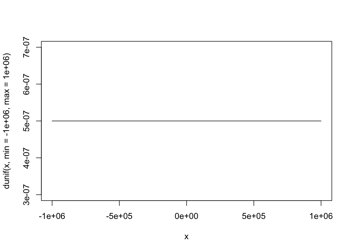
# Flat Priors
curve(dunif(x, min = -100, max = 100), from = -110, to = 110)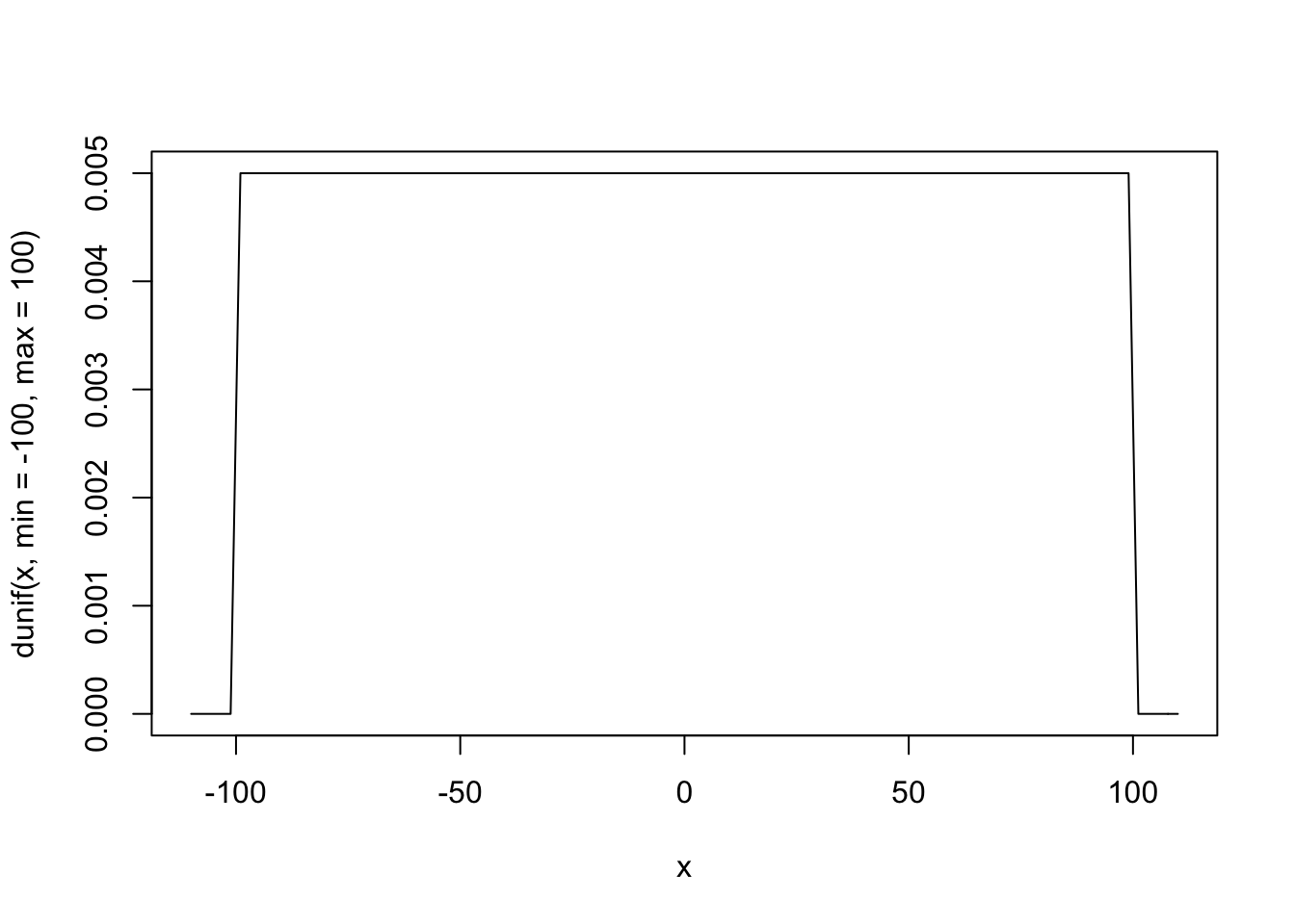
# Weakly Informative Priors
curve(dnorm(x, mean = -5, sd = 20), from = -50, to = 50)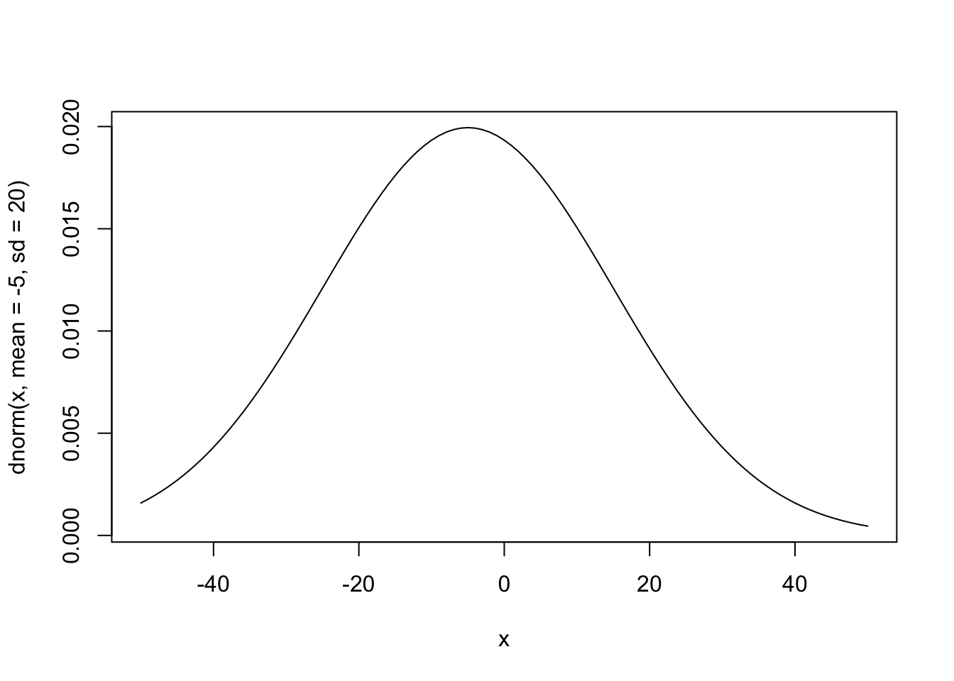
# Informative Priors
curve(dnorm(x, mean = -3, sd = 2), from = -10, to = 10)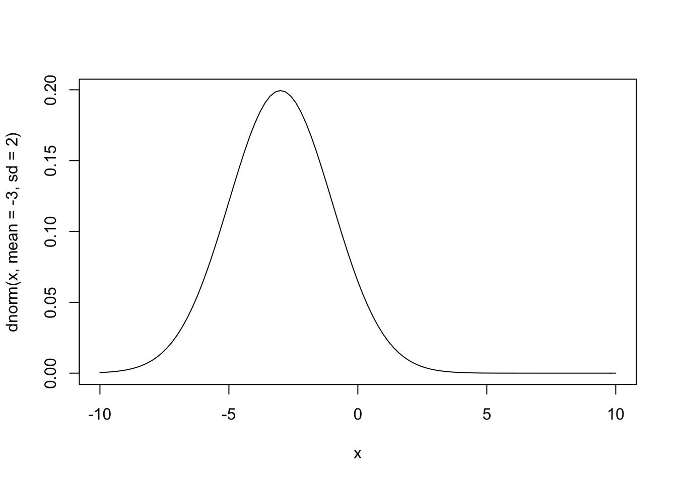
Prior Predictive Simulations
Another option for picking priors is to build a complete prior predictive simulation. Basically, this means that we run the model we are interested in without the data. To do this, we also need to pick a prior for the intercept.
To see how priors affect what the model knows we’ll look at “frequentist” priors, weakly informative priors, and very informative priors.
It’s easy to pick a prior for the intercept if we remember that the intercept is just the mean of the outcome variable. What do you think the average highway MPG is for cars in the US? 1000, -1000, 15, 30? Remember that frequentist analyses use completely uninformative priors - all values are possible.
“Frequentist” Priors
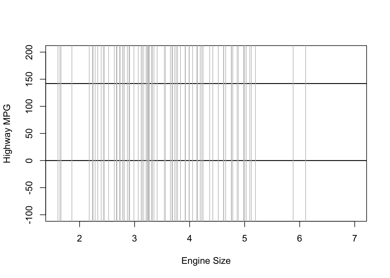
Frequentist models assume that all values are equally likely. In other words, they give no information to the model to improve prediction.
# Number of simulations
sample.size <- 100

# Prior for the intercept
intercept <- runif(sample.size, min = -10000000, max = 10000000)

# Prior for the effect of engine size
b_1 <- runif(sample.size, min = -10000000, max = 10000000)

# Variables
x <- mpg$displ
xbar <- mean(mpg$displ)

# Prior Predictive Simulation
plot(NULL, xlim = range(mpg$displ), ylim = c(-100, 200),
     xlab = "Engine Size", ylab = "Highway MPG")
abline(h = 0, lty = 1, lwd = 1.5, col = "black")
abline(h = 142, lty = 1, lwd = 1.5, col = "black")
for (i in 1:sample.size) {
  curve(intercept[i] + b_1[i] * (x - xbar), from = min(mpg$displ),
        to = max(mpg$displ), add = TRUE, col = "gray")
}
Weakly Informative Priors
Using weakly informative priors is almost always a better option. In nearly every case, we at least know something about the kind of effects/estimates we expect to find. In the example of engine size and MPG, an increase of one liter in engine size probably won’t affect highway MPG but 1,000 or even 100.
My guess is that the average car MPG is probably around 20, so we’ll use that as the mean for the prior on our intercept. Since I’m not too certain in this guess, I’ll still use a big standard deviation. As for the effect of engine size, I expect the effect to be negative and not too large so I’ll use -5 with a wide standard deviation.
# Number of simulations
sample.size <- 100

# Prior for the intercept
intercept <- rnorm(sample.size, mean = 20, sd = 20)

# Prior for the effect of engine size
b_1 <- rnorm(sample.size, mean = -5, sd = 20)

# Variables
x <- mpg$displ
xbar <- mean(mpg$displ)

# Prior Predictive Simulation
plot(NULL, xlim = range(mpg$displ), ylim = c(-100, 200),
     xlab = "Engine Size", ylab = "Highway MPG")
abline(h = 0, lty = 1, lwd = 1.5, col = "black")
abline(h = 142, lty = 1, lwd = 1.5, col = "black")
for (i in 1:sample.size) {
  curve(intercept[i] + b_1[i] * (x - xbar), from = min(mpg$displ),
        to = max(mpg$displ), add = TRUE, col = "gray")
}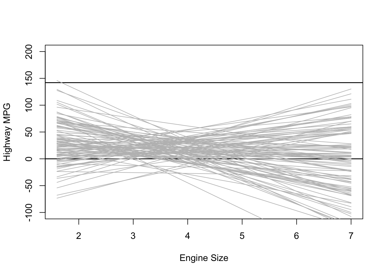
This plot shows the predicted highway MPG based only on our choice of priors for the intercept and slope. It’s not too bad, but there are definitely some outliers.
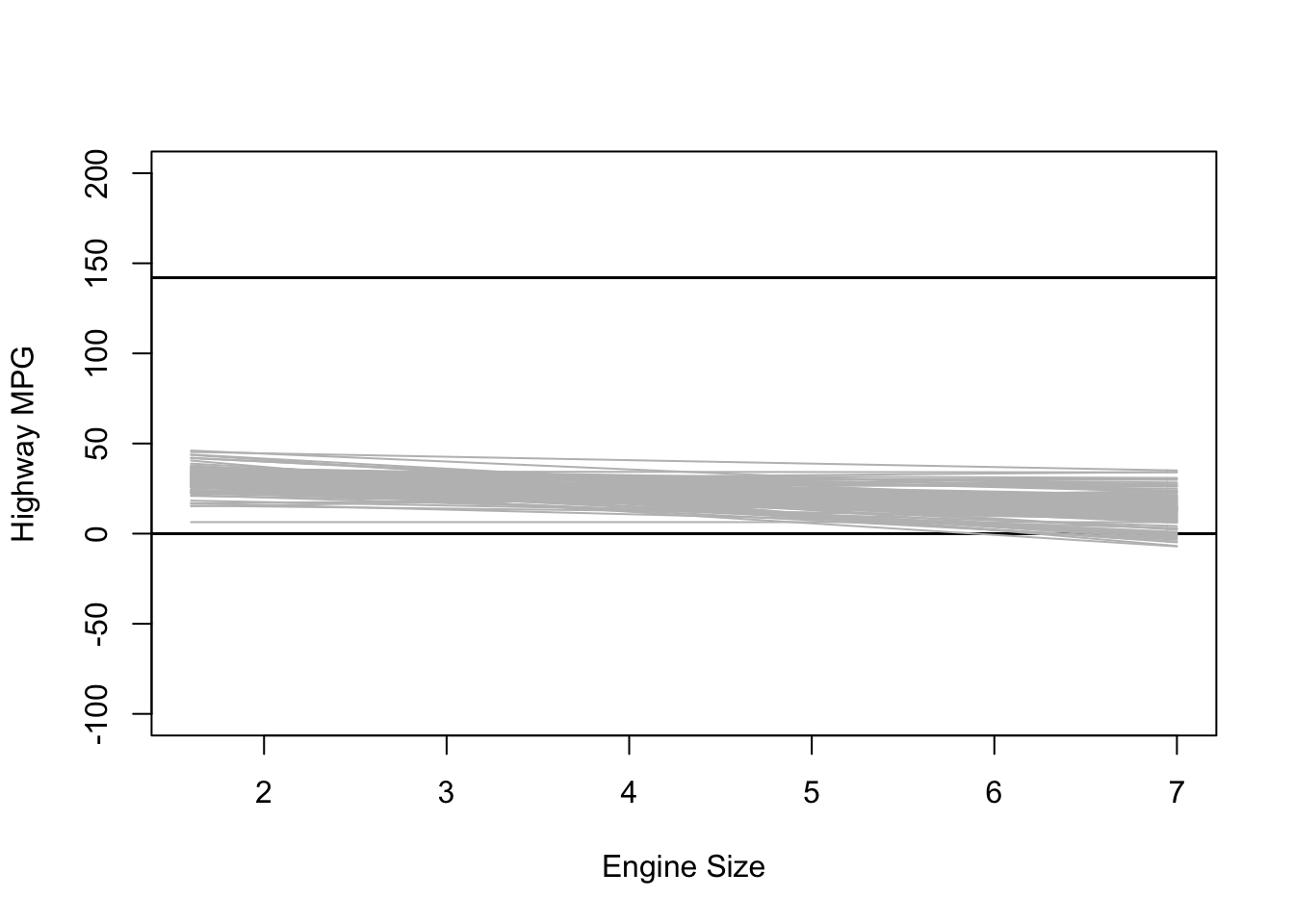
Informative Priors
What happens when we use really informative priors? Here is some data on the average MPG for different cars:

# Prior for the intercept
intercept <- rnorm(sample.size, mean = 25, sd = 5)

# Prior for the effect of engine size
b_1 <- rnorm(sample.size, mean = -3, sd = 2)

# Variables
x <- mpg$displ
xbar <- mean(mpg$displ)

# Prior Predictive Simulation
plot(NULL, xlim = range(mpg$displ), ylim = c(-100, 200),
     xlab = "Engine Size", ylab = "Highway MPG")
abline(h = 0, lty = 1, lwd = 1.5, col = "black")
abline(h = 142, lty = 1, lwd = 1.5, col = "black")
for (i in 1:sample.size) {
  curve(intercept[i] + b_1[i] * (x - xbar), from = min(mpg$displ),
        to = max(mpg$displ), add = TRUE, col = "gray")
}
Model Fitting
Now that we know what priors we want to use, we’re ready to fit the model. We’ll estimate three different models each using either “frequentist” priors, weakly informative priors, and informative priors. As a baseline, we’ll estimate the frequentist model.
# First lets create a mean centered version of displ
mpg <-
  mpg %>%
  mutate(displ_c = displ - mean(displ))

fq.fit <- glm(hwy ~ displ_c,
              family = gaussian(),
              data = mpg)
summary(fq.fit)
##
## Call:
## glm(formula = hwy ~ displ_c, family = gaussian(), data = mpg)
##
## Deviance Residuals:
## Min 1Q Median 3Q Max
## -7.1039 -2.1646 -0.2242 2.0589 15.0105
##
## Coefficients:
## Estimate Std. Error t value Pr(>|t|)
## (Intercept) 23.4402 0.2508 93.47 <2e-16 ***
## displ_c -3.5306 0.1945 -18.15 <2e-16 ***
## ---
## Signif. codes: 0 '***' 0.001 '**' 0.01 '*' 0.05 '.' 0.1 ' ' 1
##
## (Dispersion parameter for gaussian family taken to be 14.71478)
##
## Null deviance: 8261.7 on 233 degrees of freedom
## Residual deviance: 3413.8 on 232 degrees of freedom
## AIC: 1297.2
##
## Number of Fisher Scoring iterations: 2“Frequentist” Prior Model
bfit.1 <- brm(hwy ~ displ_c, # model formula
              family = gaussian(), # the likelihood function
              data = mpg, # the data the model is using
              prior = c(prior(uniform(-10000000, 10000000), class = "Intercept"),
                        prior(uniform(-10000000, 10000000), class = "b")),
              silent = 2,
              refresh = 0)
## Warning: It appears as if you have specified a lower bounded prior on a parameter that has no natural lower bound.
## If this is really what you want, please specify argument 'lb' of 'set_prior' appropriately.
## Warning occurred for prior
## b ~ uniform(-1e+07, 1e+07)## Warning: It appears as if you have specified an upper bounded prior on a parameter that has no natural upper bound.
## If this is really what you want, please specify argument 'ub' of 'set_prior' appropriately.
## Warning occurred for prior
## b ~ uniform(-1e+07, 1e+07)bfit.1## Family: gaussian
## Links: mu = identity; sigma = identity
## Formula: hwy ~ displ_c
## Data: mpg (Number of observations: 234)
## Draws: 4 chains, each with iter = 2000; warmup = 1000; thin = 1;
## total post-warmup draws = 4000
##
## Population-Level Effects:
## Estimate Est.Error l-95% CI u-95% CI Rhat Bulk_ESS Tail_ESS
## Intercept 23.44 0.25 22.93 23.92 1.00 3618 2681
## displ_c -3.53 0.20 -3.91 -3.14 1.00 3977 3043
##
## Family Specific Parameters:
## Estimate Est.Error l-95% CI u-95% CI Rhat Bulk_ESS Tail_ESS
## sigma 3.86 0.18 3.51 4.24 1.00 4212 3122
##
## Draws were sampled using sampling(NUTS). For each parameter, Bulk_ESS
## and Tail_ESS are effective sample size measures, and Rhat is the potential
## scale reduction factor on split chains (at convergence, Rhat = 1).Weakly Informative Prior Model
bfit.2 <- brm(hwy ~ displ_c, # model formula
              family = gaussian(), # the likelihood function
              data = mpg, # the data the model is using
              prior = c(prior(normal(20, 20), class = "Intercept"),
                        prior(normal(-5, 20), class = "b")),
              silent = 2,
              refresh = 0)
bfit.2
## Family: gaussian
## Links: mu = identity; sigma = identity
## Formula: hwy ~ displ_c
## Data: mpg (Number of observations: 234)
## Draws: 4 chains, each with iter = 2000; warmup = 1000; thin = 1;
## total post-warmup draws = 4000
##
## Population-Level Effects:
## Estimate Est.Error l-95% CI u-95% CI Rhat Bulk_ESS Tail_ESS
## Intercept 23.44 0.24 22.97 23.91 1.00 4227 3108
## displ_c -3.53 0.20 -3.92 -3.14 1.00 4033 2920
##
## Family Specific Parameters:
## Estimate Est.Error l-95% CI u-95% CI Rhat Bulk_ESS Tail_ESS
## sigma 3.86 0.18 3.52 4.23 1.00 4340 3160
##
## Draws were sampled using sampling(NUTS). For each parameter, Bulk_ESS
## and Tail_ESS are effective sample size measures, and Rhat is the potential
## scale reduction factor on split chains (at convergence, Rhat = 1).Informative Prior Model
bfit.3 <- brm(hwy ~ displ_c, # model formula
              family = gaussian(), # the likelihood function
              data = mpg, # the data the model is using
              prior = c(prior(normal(25, 5), class = "Intercept"),
                        prior(normal(-3, 2), class = "b")),
              silent = 2,
              refresh = 0)
bfit.3
## Family: gaussian
## Links: mu = identity; sigma = identity
## Formula: hwy ~ displ_c
## Data: mpg (Number of observations: 234)
## Draws: 4 chains, each with iter = 2000; warmup = 1000; thin = 1;
## total post-warmup draws = 4000
##
## Population-Level Effects:
## Estimate Est.Error l-95% CI u-95% CI Rhat Bulk_ESS Tail_ESS
## Intercept 23.44 0.26 22.92 23.95 1.00 3935 3135
## displ_c -3.53 0.20 -3.91 -3.13 1.00 3840 2804
##
## Family Specific Parameters:
## Estimate Est.Error l-95% CI u-95% CI Rhat Bulk_ESS Tail_ESS
## sigma 3.86 0.18 3.52 4.24 1.00 3659 3011
##
## Draws were sampled using sampling(NUTS). For each parameter, Bulk_ESS
## and Tail_ESS are effective sample size measures, and Rhat is the potential
## scale reduction factor on split chains (at convergence, Rhat = 1).Convergence Diagnostics
We always need to check the convergence of each model because they are estimated using MCMC. There are a couple ways we can check convergence. The first way is to check convergence is with a visual inspection of the traceplots. The bayesplot package makes it easy to make traceplots.
library(bayesplot)## This is bayesplot version 1.8.1## - Online documentation and vignettes at mc-stan.org/bayesplot## - bayesplot theme set to bayesplot::theme_default()## * Does _not_ affect other ggplot2 plots## * See ?bayesplot_theme_set for details on theme settingmcmc_trace(bfit.2)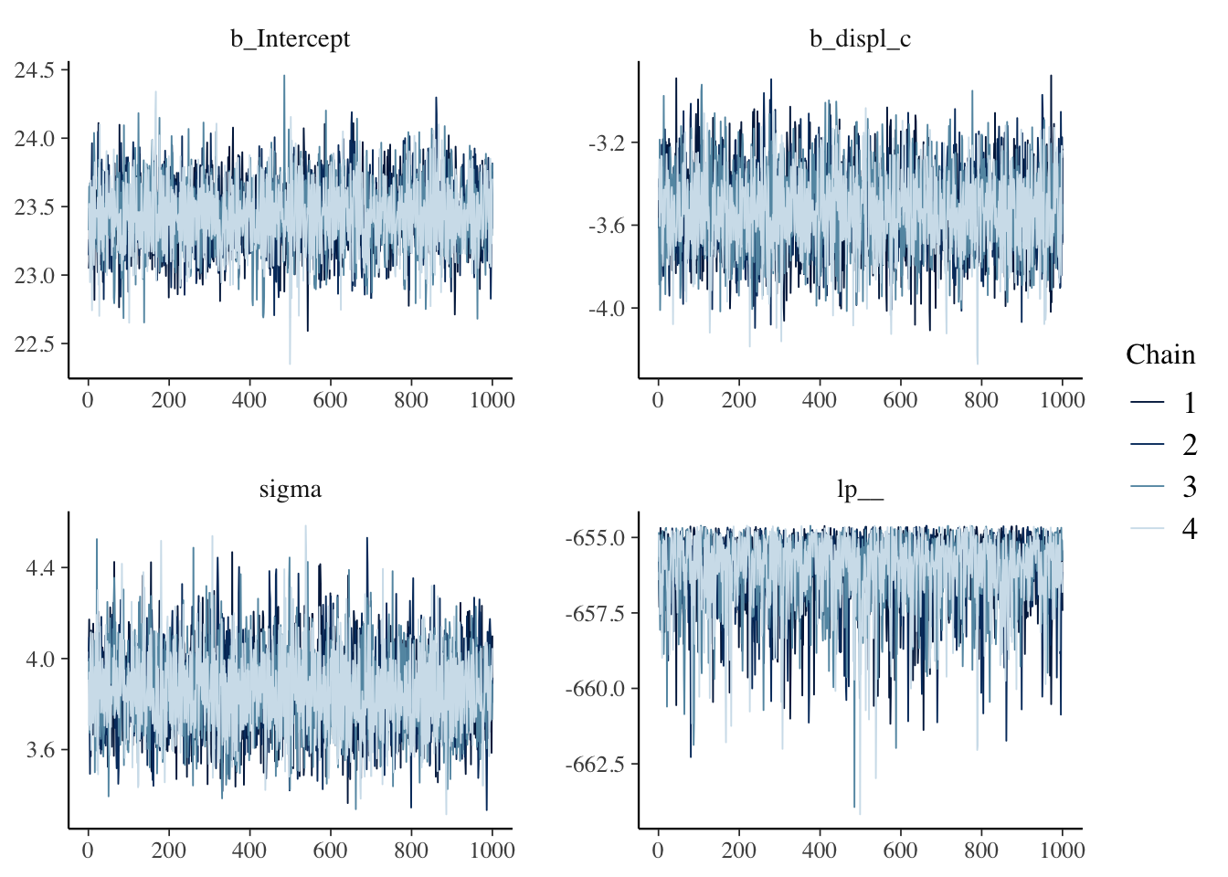
The “fuzzy caterpillar” is what we want to see. Each MCMC chain is a separate line and we want to see each line “mixing” with one another. If they will all separate that would mean that each chain has a different estimate.
Another way to check the model’s convergence is to look at the Rhat values.
bfit.2## Family: gaussian
## Links: mu = identity; sigma = identity
## Formula: hwy ~ displ_c
## Data: mpg (Number of observations: 234)
## Draws: 4 chains, each with iter = 2000; warmup = 1000; thin = 1;
## total post-warmup draws = 4000
##
## Population-Level Effects:
## Estimate Est.Error l-95% CI u-95% CI Rhat Bulk_ESS Tail_ESS
## Intercept 23.44 0.24 22.97 23.91 1.00 4227 3108
## displ_c -3.53 0.20 -3.92 -3.14 1.00 4033 2920
##
## Family Specific Parameters:
## Estimate Est.Error l-95% CI u-95% CI Rhat Bulk_ESS Tail_ESS
## sigma 3.86 0.18 3.52 4.23 1.00 4340 3160
##
## Draws were sampled using sampling(NUTS). For each parameter, Bulk_ESS
## and Tail_ESS are effective sample size measures, and Rhat is the potential
## scale reduction factor on split chains (at convergence, Rhat = 1).# rhat plot
rhats <- rhat(bfit.2)
mcmc_rhat(rhats) + xlim(1, 1.001)## Scale for 'x' is already present. Adding another scale for 'x', which will
## replace the existing scale.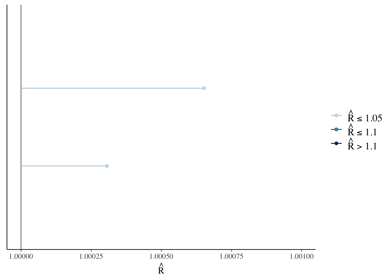
Posterior Predictive Checks
One of the unique things about Bayesian analysis is the fact that we can preform posterior predictive checks. What is a posterior predictive check? The basic idea is that if we can create a model that accurately predicts the data we have, then we should be able to use the same model to generate new data points.
pp_check(bfit.2, type = "dens_overlay", ndraws = 100)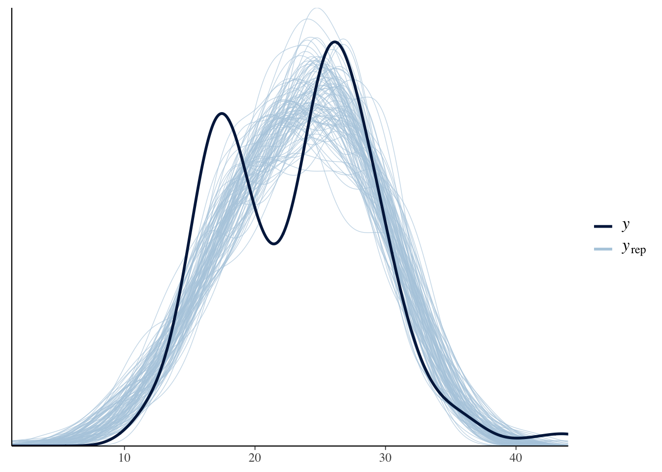
\(y\) is the actual data and \(y_{rep}\) is the data that was generated from the model. An accurate model would be able to generate new data points that follow the same distribution as the actual data. Based on this plot, it looks like we are missing some of the variation in the middle.
Results Table
library(broom.mixed)
library(knitr)
library(kableExtra)
##
## Attaching package: 'kableExtra'## The following object is masked from 'package:dplyr':
##
## group_rowsresults.table <-
tidyMCMC(bfit.3,
robust = TRUE,
conf.int = TRUE,
conf.method = "HPDinterval") %>%
mutate(conf.int = sprintf("(%.1f, %.1f)", conf.low, conf.high)) %>%
select(term, estimate, std.error, conf.int)
kable(results.table,
escape = FALSE,
booktabs = TRUE,
digits = 2,
align = c("l", "r", "r", "c"),
col.names = c("Parameter", "Point Estimate", "SD",
"95% HDI Interval ")) %>%
kable_styling(latex_options = c("striped", "hold_position"))| Parameter | Point Estimate | SD | 95% HDI Interval |
|---|---|---|---|
| b_Intercept | 23.44 | 0.26 | (23.0, 24.0) |
| b_displ_c | -3.53 | 0.20 | (-3.9, -3.1) |
| sigma | 3.86 | 0.17 | (3.5, 4.2) |
Results Visualization
Just like in frequentist statistics, we can create a coefficient plot where we see the point estimate and the 95% interval.
mcmc_plot(bfit.2, variable = "b_displ_c")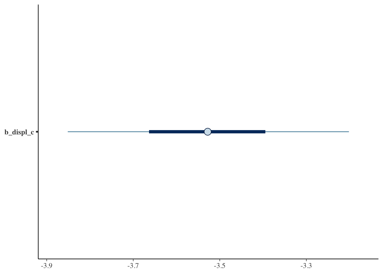
One of the best things about Bayesian analysis, however, is that we don’t just get a single point estimate. Instead we get an entire distribution of estimates. This is distribution is called the posterior distribution. We can plot it like a histogram.
mcmc_hist(bfit.2, pars = "b_displ_c")## `stat_bin()` using `bins = 30`. Pick better value with `binwidth`.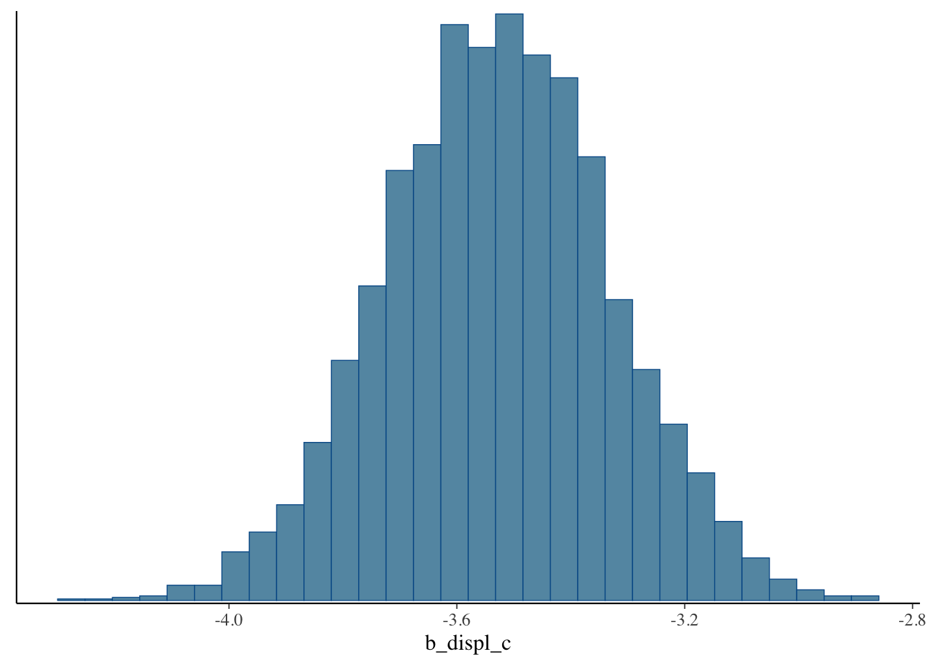
mcmc_areas(bfit.2, pars = "b_displ_c", prob = 0.95)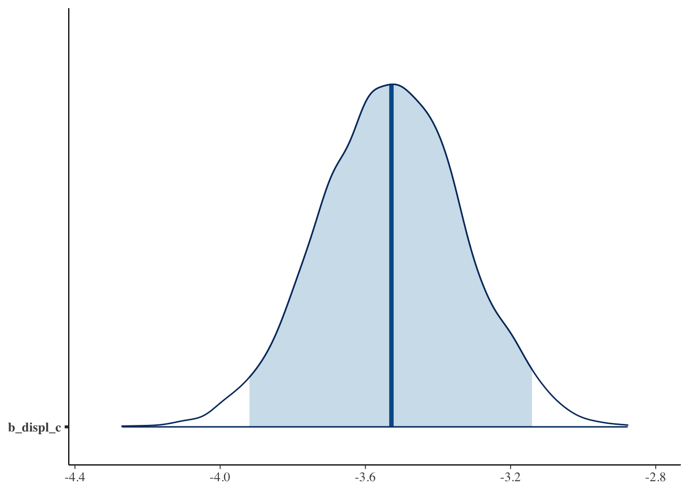
Results Interpretation
The interpretation of the results is very easy. Let’s pull them up:
bfit.2## Family: gaussian
## Links: mu = identity; sigma = identity
## Formula: hwy ~ displ_c
## Data: mpg (Number of observations: 234)
## Draws: 4 chains, each with iter = 2000; warmup = 1000; thin = 1;
## total post-warmup draws = 4000
##
## Population-Level Effects:
## Estimate Est.Error l-95% CI u-95% CI Rhat Bulk_ESS Tail_ESS
## Intercept 23.44 0.24 22.97 23.91 1.00 4227 3108
## displ_c -3.53 0.20 -3.92 -3.14 1.00 4033 2920
##
## Family Specific Parameters:
## Estimate Est.Error l-95% CI u-95% CI Rhat Bulk_ESS Tail_ESS
## sigma 3.86 0.18 3.52 4.23 1.00 4340 3160
##
## Draws were sampled using sampling(NUTS). For each parameter, Bulk_ESS
## and Tail_ESS are effective sample size measures, and Rhat is the potential
## scale reduction factor on split chains (at convergence, Rhat = 1).By default, brms shows us the mean point estimate but we could just as easily use the median or mode.
The mean point estimate is shown in the
Estimatecolumn.Est.Erroris the standard deviation of the posterior distribution.l-95% CIandu-95% CIare the lower and upper 95% credible interval estimates. Remember, the 95% credible interval tells us the range of values that will contain the true value with a 95% probability.Rhattells us about convergence. A value greater than 1.1 is bad.Bulk_ESSandTail_ESSshow the number of independent draws. The higher the better.
Read more about these things here: https://mc-stan.org/misc/warnings.html.
Let’s interpret the effect of displ_c on hwy: A one unit change in displ_c is associated with a \(-3.53\) decrease in a vehicle’s highway MPG. This effect has a standard deviation of \(0.19\) and there is a 95% probability that the true value is between \(-3.90\) and \(-3.14\).
Bonus: How Influential Are Our Priors?
To see how much our choice of priors influenced the posterior distribution we just compare the two distributions. To do this, we can draw samples from our priors when we estimate the model using the argument sample_prior = "yes". This will save the prior distributions so we can plot them later.
bfit.2 <- brm(hwy ~ displ_c, # model formula
              family = gaussian(), # the likelihood function
              data = mpg, # the data the model is using
              prior = c(prior(normal(20, 20), class = "Intercept"),
                        prior(normal(-5, 20), class = "b")),
              silent = 2,
              refresh = 0,
              sample_prior = "yes")

priors <- prior_draws(bfit.2)
head(priors)
## Intercept b sigma
## 1 27.926016 -53.173939 2.927436
## 2 33.417121 -8.934286 4.826794
## 3 7.003081 -7.465716 6.218460
## 4 14.252230 15.807468 8.453561
## 5 28.373259 14.919524 16.521201
## 6 -25.861000 -2.497979 10.068648This shows all 4,000 draws from the priors that we used. If we summarize them, we’ll see that the mean is just about equal to what we set it to.
summary(priors)## Intercept b sigma
## Min. :-49.913 Min. :-70.105 Min. : 0.00008
## 1st Qu.: 6.766 1st Qu.:-18.831 1st Qu.: 2.67372
## Median : 20.292 Median : -5.710 Median : 5.88203
## Mean : 20.202 Mean : -5.543 Mean : 8.29821
## 3rd Qu.: 33.768 3rd Qu.: 7.688 3rd Qu.: 10.61485
## Max. : 90.531 Max. : 65.585 Max. :234.76037Now we can plot them:
ggplot() +
  geom_density(data = priors, aes(x = b)) +
  labs(title = "Prior Distribution") +
  theme_classic()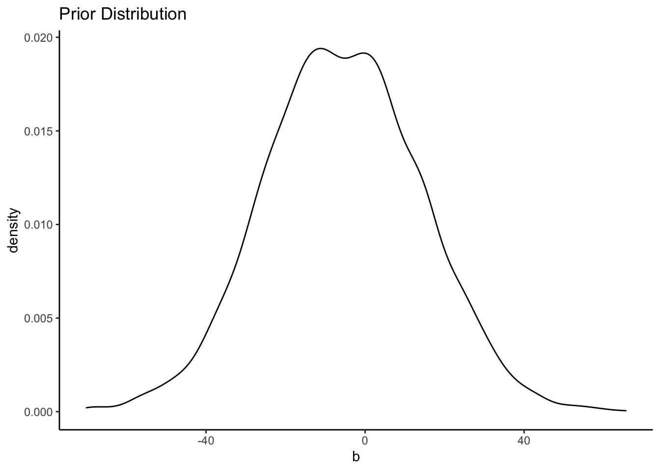
We can also plot the posterior distribution:
posteriors <- as.data.frame(bfit.2)

ggplot() +
  geom_density(data = posteriors, aes(x = b_displ_c), color = "blue") +
  labs(title = "Posterior Distribution") +
  theme_classic()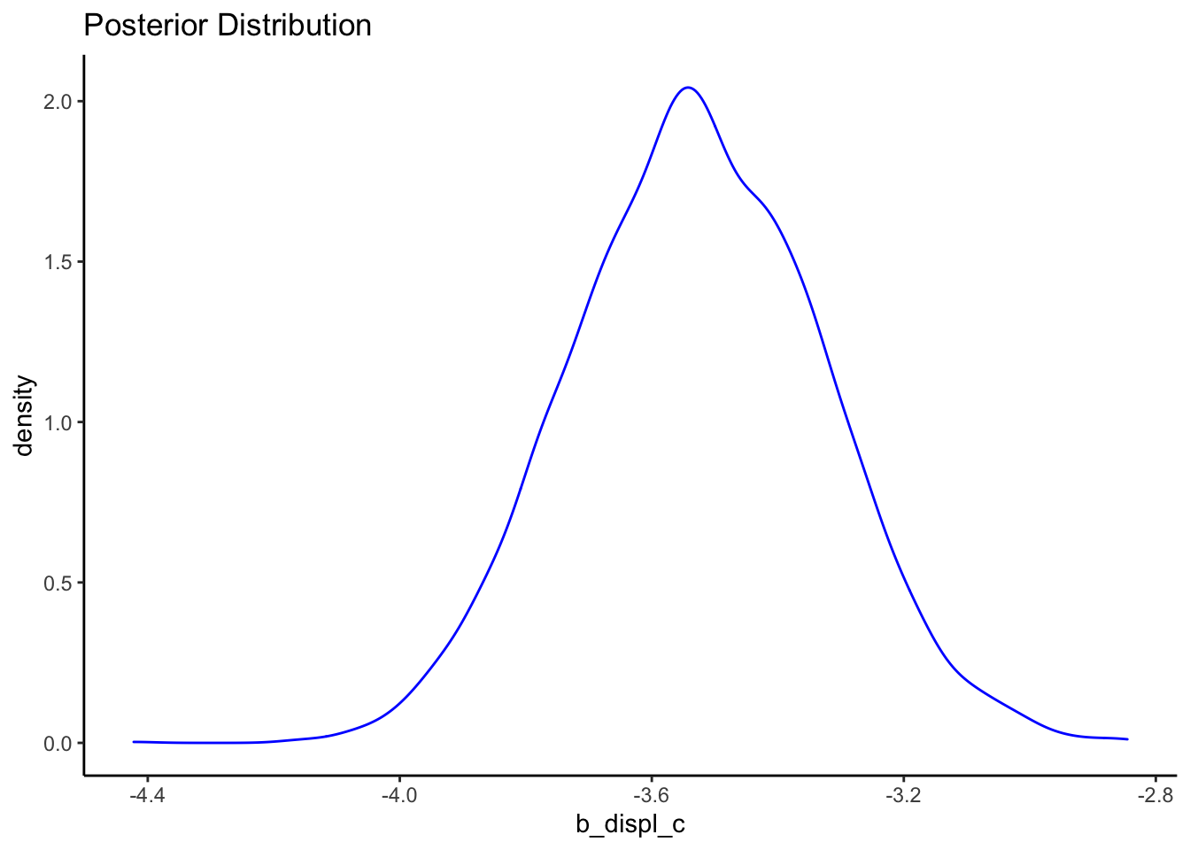
It’s easy to see the comparison of the prior distribution to the posterior if we put them on the same plot. Since the x-axes are so different, however, we’ll need to make some manual adjustments.
ggplot() +
  geom_density(data = priors, aes(x = b)) +
  geom_density(data = posteriors, aes(x = b_displ_c), color = "blue") +
  labs(title = "Prior Distribution vs. Posterior Distribution") +
  xlim(-10, 10) +
  theme_classic()
## Warning: Removed 2542 rows containing non-finite values (stat_density).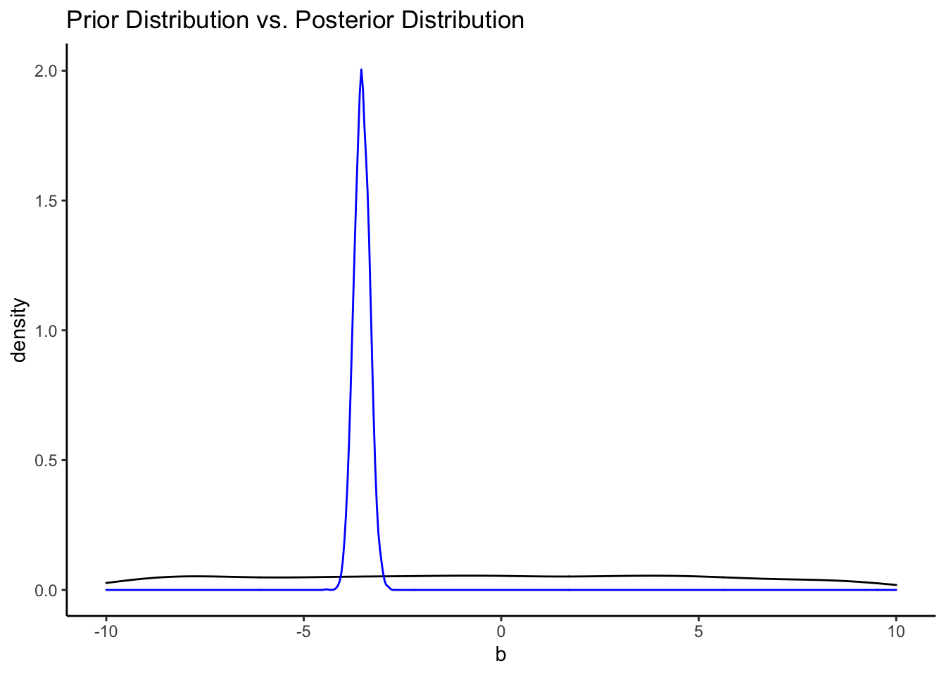
That’s a pretty uninformative prior. How do the priors from the informative model compare?
bfit.3 <- brm(hwy ~ displ_c, # model formula
              family = gaussian(), # the likelihood function
              data = mpg, # the data the model is using
              prior = c(prior(normal(25, 5), class = "Intercept"),
                        prior(normal(-3, 2), class = "b")),
              silent = 2,
              refresh = 0,
              sample_prior = "yes")

priors <- prior_draws(bfit.3)
posteriors <- as.data.frame(bfit.3)

ggplot() +
  geom_density(data = priors, aes(x = b)) +
  geom_density(data = posteriors, aes(x = b_displ_c), color = "blue") +
  labs(title = "Prior Distribution vs. Posterior Distribution") +
  xlim(-10, 10) +
  theme_classic()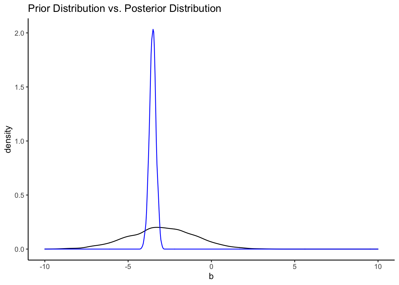
Resources
Looking to learn more about all of this Bayesian stuff? I recommend the following resources: