Data Cleaning
We’ll be using R Studio for our workshop because it provides convenient support for both R and Python. It also provides an awesome visual markdown editor which allows you to see your markdown syntax compiled in real time.
Markdown is arguably THE best tool for reporting results and we will be making use of it during this workshop series. In the final workshop, we’ll learn how we can use markdown to write dynamic documents, which are documents where you write up the results of your research with your code to produce all figures, tables, and models at the same time. Writing the code and prose together makes it easy to modify your report if the analysis changes, minimizes errors, and it also encourages reproducibility since readers can find your code in the body of the text. But, all that is for another day. For now, let’s focus on data exploration.
Session Learning Objectives
Work with RMarkdown to write code and report results
Learn the basics of R and refresh your Python skills
Clean a dataset for analysis
- Handle missing values
- Rename variables
- Create variables
- Pivot Data
- Separate Data
Learn the “tidy data” phlisophy
(R)Markdown Refresher
You create the biggest header using the # sign.
This is a smaller header
This is an even smaller header
… you get it
This makes a bullet point
What about a numbered list?
- Just use numbers…
Viewing Markdown
How can we see what this will look like when it’s rendered? RStudio gives us two options. First, we can Knit the document by clicking the button on the tool bar that looks like this:
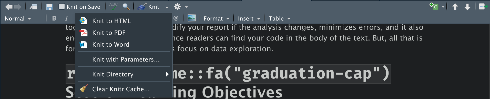
Knitting to an HTML file is easiest, but as you can see, if you click on the drop down arrow to the right of Knit, you get more output options. Knit works by calling Pandoc on the backend to render your markdown file into the output that you want.
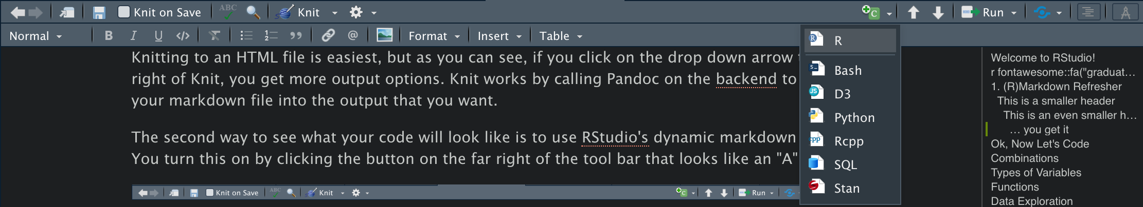
The second way to see what your code will look like is to use R Studio’s dynamic markdown editor. You turn this on by clicking the button on the far right of the tool bar that looks like an “A”:

The last markdown tool you should know about for now, is that RStudio lets you see the document outline which can be helpful when writing a long document. To see it, click the button just to the left of the dynamic editor button:

Onwards!
To start a codeblock (where you would write code), you use three tick marks ``` followed by the language you want to write in curly brackets {} like this: ```{r}. To close the block, you enter three tick marks on the line below (note that you have to have a space in between the start of the block and the end) ```.
Instead of adding a block manually, you can also use the little green insert button on the tool bar:
Learning R and Refreshing Python
R is just a really fancy calculator. Python is more general, but it can still preform the same calculations that R can. Let’s start with some basic math in Python. To start, insert a Python code chunk:
# let's start with addition
1 + 1
## 25 + 2
# notice the spaces between the + operator. This is considered good grammar.
# It's a lot harder to read without spaces (it gets worse when we have
# complex code).## 71+1 # bad## 25+2 # bad
# multiplication## 74 * 8## 325 * 19
# division## 954 / 8## 0.514 / 7
# power functions## 2.04 ** 2## 16Now let’s reproduce this in R:
# addition
1 + 1
## [1] 25 + 2## [1] 7# multiplication
4 * 8## [1] 325 * 19## [1] 95# division
4 / 8## [1] 0.514 / 7## [1] 2# cubes
4 ^ 2## [1] 16Everything was the same with the exception of the power function at the end. R using ^ and Python uses **.
The answers to each problem are shown at the bottom of the code block, but what if we wanted to save the answer to retrieve it later? This is where to concept of assignment comes in. When we make an assignment, we are creating an object that holds whatever we tell it to. In Python it looks like this:
answer = 5 + 2

# again, note the spacing above. The spacing below is bad:
answer=5+2 # bad
Now, if we want to see the answer to our operation, we just print the object we saved it to: answer:
answer## 7Assignment works nearly the same way in R. The main difference is with the assignment operator. While the = works for assignment in R, it’s considered bad practice to use it for assignment. Instead we use <- when making an assignment.
answer <- 5 + 2
answer
## [1] 7The second different is that when making an assignment, R creates a copy
If you look in the environment pane, you will see the object (answer) that we created. You might also notice that the top left corner of the environment pane says R. If you click that, you’ll see that you can also select Python to see all of the Python objects you’ve created.
Exercises
- Insert a Python code chunk and calculate \(17 \times 6\). Assign your answer to an object named
answer2. - Now do the same in R.
Lists and Vectors
What if we wanted to combine several operations in one object? In Python, we accomplish this by creating a list:
a = [1, 2, 3]
a
## [1, 2, 3]In R, we create a list with the c function and parentheses ().
a <- c(1, 2, 3)
a
## [1] 1 2 3# we can include text instead of numbers and operations. Put text in quotations
text <- c("This", "Shows", "That we can also have text")
print(text)## [1] "This" "Shows"
## [3] "That we can also have text"In R, we mainly refer to these as vectors. Like Python, lists can contain text, text and numbers, or operations
text <- c("This", "Shows", "That we can also have text")
text
## [1] "This" "Shows"
## [3] "That we can also have text"b <- c(2, 5, "Text")
b## [1] "2" "5" "Text"c <- c(3 + 3, 4 * 8, 17)
c## [1] 6 32 17Types of Variables
When you work with data, chances are you’ll working with many different types of data at the same time. Consider this pandas DataFrame:
import pandas as pd

data = pd.DataFrame(
  {"age": [33, 24, 42, 20, 19, 23],
   "education": ["High School", "Bachelors", "Bachelors", "High School",
                 "Some College", "Grad School"],
   "surname": ["smith", "gonzales", "lee", "doe", "kim", "swanson"]}
)

data
## age education surname
## 0 33 High School smith
## 1 24 Bachelors gonzales
## 2 42 Bachelors lee
## 3 20 High School doe
## 4 19 Some College kim
## 5 23 Grad School swansonHere we have three different types of data. age is clearly numeric and education and surname are strings. But, is there a difference between education and surname? education is best considered a categorical variable because each level of education is a different category. surname of the other hand isn’t really categorical, it’s just text.
We can check the data types of the DataFrame in Python like this:
data.dtypes## age int64
## education object
## surname object
## dtype: objectFor reasons that I won’t explain here, pandas uses the type “object” for strings, so this is correct. What about with R? To recreate this data frame in R we use the data.frame function:
r.data <- data.frame(
  age = c(33, 24, 42, 20, 19, 23),
  education = c("High School", "Bachelors", "Bachelors", "High School",
                "Some College", "Grad School"),
  surname = c("smith", "gonzales", "lee", "doe", "kim", "swanson")
)

head(r.data)
## age education surname
## 1 33 High School smith
## 2 24 Bachelors gonzales
## 3 42 Bachelors lee
## 4 20 High School doe
## 5 19 Some College kim
## 6 23 Grad School swansonThe head() function shows the first 6 rows of data and at the top of each column you see the data type. It shows that age is of type <dbl> which stands for double and basically means that it’s numeric data. education and surname are of type <chr> which means character, or string.
Earlier, I said that education should be a category, so why isn’t it? R and Python can’t really recognize the difference between strings and categories so we have to manually set it.
In Python, we can convert education to a categorical type with the .astype("category") method:
data["education"].astype("category")## 0 High School
## 1 Bachelors
## 2 Bachelors
## 3 High School
## 4 Some College
## 5 Grad School
## Name: education, dtype: category
## Categories (4, object): ['Bachelors', 'Grad School', 'High School', 'Some College']Now in R:
r.data["education"] <- as.factor(r.data$education)
head(r.data)
## age education surname
## 1 33 High School smith
## 2 24 Bachelors gonzales
## 3 42 Bachelors lee
## 4 20 High School doe
## 5 19 Some College kim
## 6 23 Grad School swansonIn this R block, we used a new operator $. This operator allows us to access columns of a data frame. In an R block, try typing: r.data$ then hit the Tab key. All of the columns are listed out. You can use the arrow keys to navigate to the one you want and hit Tab again.
Setting your data types correctly is an important aspect of data cleaning because it will make data visualization and analysis much easier down the line.
You can convert (also known as casting or coercing) a data frame column to other types data as well. These include numeric, character, integers, datetimes and more.
Exercises
- Use R to coerce the
agevariable inr.datato an integer. - Use Python cast the
agevariable as an integer. (Hint: the integer type in Python isint64)
Getting Help!
Like the Python, the help options in R are very useful. If you place a ? before any function, it will pull up a help menu:
?mean()Exercise
- Create this vector in R:
vector <- c(123, 45, NA, 78, 17), the find the mean.
Clean a Dataset for Analysis
Data cleaning (munging, or wrangling) is the primary task of any data science project. Data is really great for improving decisions, but only if it is in a usable format and only if we know what the data is measuring. There are a lot of different tasks involved in data cleaning, and in this workshop we will focus on three of the most important tasks:
- Handling missing data
- Renaming variables
- Creating dummy variables
To see all of these tasks in action, lets get started with an actual dataset. The dataset that we’ll being using for the remainder of this workshop is about flights to and from various destinations. Let’s load it in with Python:
flights_data = pd.read_csv("https://raw.githubusercontent.com/vaibhavwalvekar/NYC-Flights-2013-Dataset-Analysis/master/flights.csv")

flights_data.head()
## Unnamed: 0 year month day ... air_time distance hour minute
## 0 1 2013 1 1 ... 227.0 1400 5.0 17.0
## 1 2 2013 1 1 ... 227.0 1416 5.0 33.0
## 2 3 2013 1 1 ... 160.0 1089 5.0 42.0
## 3 4 2013 1 1 ... 183.0 1576 5.0 44.0
## 4 5 2013 1 1 ... 116.0 762 5.0 54.0
##
## [5 rows x 17 columns]Note that would can also load this data into R in a very similar way. First we’ll load the tidyverse package, then load the data:
library(tidyverse)## ── Attaching packages ─────────────────────────────────────── tidyverse 1.3.1 ──## ✓ ggplot2 3.3.5 ✓ purrr 0.3.4
## ✓ tibble 3.1.6 ✓ dplyr 1.0.8
## ✓ tidyr 1.2.0 ✓ stringr 1.4.0
## ✓ readr 2.1.2 ✓ forcats 0.5.1## ── Conflicts ────────────────────────────────────────── tidyverse_conflicts() ──
## x dplyr::filter() masks stats::filter()
## x dplyr::lag() masks stats::lag()flights <- read_csv("https://raw.githubusercontent.com/vaibhavwalvekar/NYC-Flights-2013-Dataset-Analysis/master/flights.csv")## New names:
## * `` -> ...1## Rows: 336776 Columns: 17
## ── Column specification ────────────────────────────────────────────────────────
## Delimiter: ","
## chr (4): carrier, tailnum, origin, dest
## dbl (13): ...1, year, month, day, dep_time, dep_delay, arr_time, arr_delay, ...
##
## ℹ Use `spec()` to retrieve the full column specification for this data.
## ℹ Specify the column types or set `show_col_types = FALSE` to quiet this message.head(flights)## # A tibble: 6 × 17
## ...1 year month day dep_time dep_delay arr_time arr_delay carrier tailnum
## <dbl> <dbl> <dbl> <dbl> <dbl> <dbl> <dbl> <dbl> <chr> <chr>
## 1 1 2013 1 1 517 2 830 11 UA N14228
## 2 2 2013 1 1 533 4 850 20 UA N24211
## 3 3 2013 1 1 542 2 923 33 AA N619AA
## 4 4 2013 1 1 544 -1 1004 -18 B6 N804JB
## 5 5 2013 1 1 554 -6 812 -25 DL N668DN
## 6 6 2013 1 1 554 -4 740 12 UA N39463
## # … with 7 more variables: flight <dbl>, origin <chr>, dest <chr>,
## # air_time <dbl>, distance <dbl>, hour <dbl>, minute <dbl>Of course, the read functions in Python and R also accept traditional file paths and file names instead of URLs like this:
read_csv("Documents/my_project/data.csv")And, you can read in many other types of data with Python and R. Here is a table that shows the functions needed to read in other common file types:
| File Type | R Function | Python Function |
|---|---|---|
| CSV | readr::read_csv |
pandas.read_csv |
Excel (.xls & .xlsx) |
readxl::read_excel |
pandas.read_excel |
| SPSS | haven::read_spss |
pandas.read_spss |
| Stata | haven::read_dta |
pandas.read_stata |
| SAS | haven::read_sas |
pandas.read_sas |
| Feather | feather::read_feather |
pandas.read_feather |
The beauty of using a tool like RStudio is that we don’t have to only use R or only use Python. RStudio lets us use both languages to work with the same data. This is made possible by the reticulate package in R. After we load it in, we can use R and Python to interact with the same data. This is how it works:
library(reticulate) # load the reticulate package

# to pull data loaded with Python in R, just use the preface py$
head(py$flights_data)
## Unnamed: 0 year month day dep_time dep_delay arr_time arr_delay carrier
## 1 1 2013 1 1 517 2 830 11 UA
## 2 2 2013 1 1 533 4 850 20 UA
## 3 3 2013 1 1 542 2 923 33 AA
## 4 4 2013 1 1 544 -1 1004 -18 B6
## 5 5 2013 1 1 554 -6 812 -25 DL
## 6 6 2013 1 1 554 -4 740 12 UA
## tailnum flight origin dest air_time distance hour minute
## 1 N14228 1545 EWR IAH 227 1400 5 17
## 2 N24211 1714 LGA IAH 227 1416 5 33
## 3 N619AA 1141 JFK MIA 160 1089 5 42
## 4 N804JB 725 JFK BQN 183 1576 5 44
## 5 N668DN 461 LGA ATL 116 762 5 54
## 6 N39463 1696 EWR ORD 150 719 5 54From now on we’ll only be using the flights_data that we imported with Python. We’ll also start to slowly transition to using R over Python.
Missing Data
It’s important to handle missing data correctly because missing values can influence analyses.
There are two types of missing data. The first is called “explicitly” missing data. Explicitly missing data values show up in R or Python as NA or NaN and these values tell you that there is no data for a given cell. Here is an example:
df <- tibble(
  state = c("CA", "CA", "AZ", "AZ", "TX", "TX"),
  year = c(2000, 2001, 2000, 2001, 2000, 2001),
  enrollments = c(1521, 1231, 3200, 2785, 6731, NA)
)
df
## # A tibble: 6 × 3
## state year enrollments
## <chr> <dbl> <dbl>
## 1 CA 2000 1521
## 2 CA 2001 1231
## 3 AZ 2000 3200
## 4 AZ 2001 2785
## 5 TX 2000 6731
## 6 TX 2001 NAIt’s clear that there is no data for Texas in 2001. But, what if there just was no row of data instead of an NA value? For example:
df <- tibble(
  state = c("CA", "CA", "AZ", "AZ", "TX"),
  year = c(2000, 2001, 2000, 2001, 2000),
  enrollments = c(1521, 1231, 3200, 2785, 6731)
)
df
## # A tibble: 5 × 3
## state year enrollments
## <chr> <dbl> <dbl>
## 1 CA 2000 1521
## 2 CA 2001 1231
## 3 AZ 2000 3200
## 4 AZ 2001 2785
## 5 TX 2000 6731This would be known as an “implicitly” missing value. We don’t have the data for Texas which, by definition, means that it’s missing, but it’s not explicit in the data. If we wanted to make it explicit, we could use the complete() function which fills out all possible values for a combination of variables:
complete(df, state, year)## # A tibble: 6 × 3
## state year enrollments
## <chr> <dbl> <dbl>
## 1 AZ 2000 3200
## 2 AZ 2001 2785
## 3 CA 2000 1521
## 4 CA 2001 1231
## 5 TX 2000 6731
## 6 TX 2001 NASometimes explicitly missing values are coded as -99 or -999 and that can affect statistical summaries like the mean, median, and even correlations.
Both R and Python have default ways of handling missing values. In R, they are displayed as NA and in Python as NaN. Let’s see an example of this:
flights_data## Unnamed: 0 year month day ... air_time distance hour minute
## 0 1 2013 1 1 ... 227.0 1400 5.0 17.0
## 1 2 2013 1 1 ... 227.0 1416 5.0 33.0
## 2 3 2013 1 1 ... 160.0 1089 5.0 42.0
## 3 4 2013 1 1 ... 183.0 1576 5.0 44.0
## 4 5 2013 1 1 ... 116.0 762 5.0 54.0
## ... ... ... ... ... ... ... ... ... ...
## 336771 336772 2013 9 30 ... NaN 213 NaN NaN
## 336772 336773 2013 9 30 ... NaN 198 NaN NaN
## 336773 336774 2013 9 30 ... NaN 764 NaN NaN
## 336774 336775 2013 9 30 ... NaN 419 NaN NaN
## 336775 336776 2013 9 30 ... NaN 431 NaN NaN
##
## [336776 rows x 17 columns]What columns have missing values?
In Python we can calculate this by pairing .isnull() and .any() methods:
flights_data.isnull().any()## Unnamed: 0 False
## year False
## month False
## day False
## dep_time True
## dep_delay True
## arr_time True
## arr_delay True
## carrier False
## tailnum True
## flight False
## origin False
## dest False
## air_time True
## distance False
## hour True
## minute True
## dtype: boolHere we see that quite a few variables have missing values.
How many missing values are there?
flights_data.isnull().sum()## Unnamed: 0 0
## year 0
## month 0
## day 0
## dep_time 8255
## dep_delay 8255
## arr_time 8713
## arr_delay 9430
## carrier 0
## tailnum 2512
## flight 0
## origin 0
## dest 0
## air_time 9430
## distance 0
## hour 8255
## minute 8255
## dtype: int64We could replicate this with R code, by Python provides pretty good tools to answer these questions.
Next, let’s look at the summary statistics for our data to check for any unusual values:
flights_data.describe()## Unnamed: 0 year ... hour minute
## count 336776.000000 336776.0 ... 328521.000000 328521.000000
## mean 168388.500000 2013.0 ... 13.173544 31.755501
## std 97219.001466 0.0 ... 4.894426 18.230997
## min 1.000000 2013.0 ... 0.000000 0.000000
## 25% 84194.750000 2013.0 ... 9.000000 16.000000
## 50% 168388.500000 2013.0 ... 14.000000 31.000000
## 75% 252582.250000 2013.0 ... 17.000000 49.000000
## max 336776.000000 2013.0 ... 24.000000 59.000000
##
## [8 rows x 13 columns]What should we do with missing values?
There really isn’t a “right” way to handle missing values, so you just need to think carefully about whatever decision you make. The solution that we’ll use here is just to drop all missing values. Why? Missing values can’t be put in a plot or used in a regression, so we don’t necessarily need them. Theoretically, missing values are important because it could mean something more that just “no data.” For example, data might be systematically missing for a particular group of people. That would definitely affect our analyses and we would want to address it. That’s a very different situation than having a missing value for a random, non-systematic reason.
Now that we’ve seen a small comparison of Python with R, we’re going to start primarily using R to do the rest of our cleaning and exploration. We’ll be using R’s tidyverse specifically, which is a collection of packages that make R syntax easy to read, easy to type, and powerful.
So, let’s drop all missing values, understanding that such a decision many not be the best for all situations. We’ll accomplish this with the drop_na() function provided by the dplyr R package (one of the packages included in the tidyverse). We’re also going to create a new object to save our changes to so that we can start building the dataset that we need to analysis and so that we can get back to our original data if needed.
flights_no_na <- drop_na(py$flights_data)How many rows did we drop? Let’s check:
# before dropping NAs
nrow(py$flights_data)
## [1] 336776# after dropping NAs
nrow(flights_no_na)## [1] 327346# total rows dropped
nrow(py$flights_data) - nrow(flights_no_na)## [1] 9430Let’s use Python to confirm that we dropped all missing values:
r.flights_no_na.isnull().any()## Unnamed: 0 False
## year False
## month False
## day False
## dep_time False
## dep_delay False
## arr_time False
## arr_delay False
## carrier False
## tailnum False
## flight False
## origin False
## dest False
## air_time False
## distance False
## hour False
## minute False
## dtype: boolLooks good!
Renaming Variables
Another common data cleaning task is to rename variables. Sometimes variable names are completely uninformative - something like CMP23A_001. That doesn’t make it any easier to understand the data. Let’s check out the names of our variables in our dataset:
colnames(flights_no_na)## [1] "Unnamed: 0" "year" "month" "day" "dep_time"
## [6] "dep_delay" "arr_time" "arr_delay" "carrier" "tailnum"
## [11] "flight" "origin" "dest" "air_time" "distance"
## [16] "hour" "minute"These are actually pretty good, but we’ll make some changes anyway. Most of our variable names have a _ separator when they involve two words. tailnum is the exception. Let’s rename this variable to tail_num.
To do this, we’re going to make use of the “pipe” operator: %>%. This is a special operator that is used to chain multiple functions together. Chaining functions allows us to execute several operations quickly. I’ll right out the code to rename tailnum below with comments to teach you what each step is doing:
# first we make an assignment to save our changes
# since we want to use the same object name, we'll assign all of our changes to it
# this first line can be read aloud as: "create an object named 'flights_no_na'
# using the existing object 'flights_no_na' THEN ...
flights_no_na <- flights_no_na %>%
  # rename NEW NAME = OLD NAME
  rename(tail_num = tailnum)

colnames(flights_no_na)
## [1] "Unnamed: 0" "year" "month" "day" "dep_time"
## [6] "dep_delay" "arr_time" "arr_delay" "carrier" "tail_num"
## [11] "flight" "origin" "dest" "air_time" "distance"
## [16] "hour" "minute"We’ll also use this opportunity to drop the variable Unnamed: 0 since it doesn’t appear to contain any useful information. We can drop a variable with the select() function. select() is used to pick out only the variables that we want like this:
flights_no_na %>%
  select(origin, dest) %>%
  head()
## origin dest
## 1 EWR IAH
## 2 LGA IAH
## 3 JFK MIA
## 4 JFK BQN
## 5 LGA ATL
## 6 EWR ORDHere I only selected the origin and dest variables but I made no assignment. That means that I didn’t make any changes to the flights_no_na data frame. See:
head(flights_no_na)## Unnamed: 0 year month day dep_time dep_delay arr_time arr_delay carrier
## 1 1 2013 1 1 517 2 830 11 UA
## 2 2 2013 1 1 533 4 850 20 UA
## 3 3 2013 1 1 542 2 923 33 AA
## 4 4 2013 1 1 544 -1 1004 -18 B6
## 5 5 2013 1 1 554 -6 812 -25 DL
## 6 6 2013 1 1 554 -4 740 12 UA
## tail_num flight origin dest air_time distance hour minute
## 1 N14228 1545 EWR IAH 227 1400 5 17
## 2 N24211 1714 LGA IAH 227 1416 5 33
## 3 N619AA 1141 JFK MIA 160 1089 5 42
## 4 N804JB 725 JFK BQN 183 1576 5 44
## 5 N668DN 461 LGA ATL 116 762 5 54
## 6 N39463 1696 EWR ORD 150 719 5 54All the variables are still there!
Now, to drop Unnamed: 0 we can use a minus sign - in the select function like this:
flights_no_na %>%
  select(-`Unnamed: 0`) %>%
  head()
## year month day dep_time dep_delay arr_time arr_delay carrier tail_num flight
## 1 2013 1 1 517 2 830 11 UA N14228 1545
## 2 2013 1 1 533 4 850 20 UA N24211 1714
## 3 2013 1 1 542 2 923 33 AA N619AA 1141
## 4 2013 1 1 544 -1 1004 -18 B6 N804JB 725
## 5 2013 1 1 554 -6 812 -25 DL N668DN 461
## 6 2013 1 1 554 -4 740 12 UA N39463 1696
## origin dest air_time distance hour minute
## 1 EWR IAH 227 1400 5 17
## 2 LGA IAH 227 1416 5 33
## 3 JFK MIA 160 1089 5 42
## 4 JFK BQN 183 1576 5 44
## 5 LGA ATL 116 762 5 54
## 6 EWR ORD 150 719 5 54A couple things to note here. First, I made no assignment so I didn’t save our changes (i.e. Unnamed: 0 is still in our original data frame). Second, check out the `` marks around Unnamed: 0. We need those because Unnamed: 0 has white space and that makes R mad.
With all that in mind, let’s drop Unnamed: 0 once and for all by including an assignment in our code:
flights_no_na <- flights_no_na %>%
  select(-`Unnamed: 0`)
Exercise
- Rename
destasdestination.
Creating Variables
Creating variables is easy with the mutate() function. Say we want to create a new variable that calculates the total delay (tot_delay) that is the sum of the departure delay (dep_delay) and the arrival delay (arr_delay) of each flight:
flights_no_na <- flights_no_na %>%
  mutate(tot_delay = dep_delay + arr_delay)
We can create more that one variable at a time like this:
flights_no_na <- flights_no_na %>%
  mutate(tot_delay = dep_delay + arr_delay,
         tot_delay_alt  = (dep_delay + arr_delay) / 60)
mutate() can also be used to modify existing variables. For example, suppose we wanted to convert carrier to be a categorical type of data:
flights_no_na <- flights_no_na %>%
  mutate(carrier = as.factor(carrier))

head(flights_no_na)
## year month day dep_time dep_delay arr_time arr_delay carrier tail_num flight
## 1 2013 1 1 517 2 830 11 UA N14228 1545
## 2 2013 1 1 533 4 850 20 UA N24211 1714
## 3 2013 1 1 542 2 923 33 AA N619AA 1141
## 4 2013 1 1 544 -1 1004 -18 B6 N804JB 725
## 5 2013 1 1 554 -6 812 -25 DL N668DN 461
## 6 2013 1 1 554 -4 740 12 UA N39463 1696
## origin dest air_time distance hour minute tot_delay
## 1 EWR IAH 227 1400 5 17 13
## 2 LGA IAH 227 1416 5 33 24
## 3 JFK MIA 160 1089 5 42 35
## 4 JFK BQN 183 1576 5 44 -19
## 5 LGA ATL 116 762 5 54 -31
## 6 EWR ORD 150 719 5 54 8Exercise
- Use
mutate()to compute the total air time for each flight (Hint: usedep_timeandarr_time). Does this value equal the value inair_time. Why or why not?
The “tidy data” Philosophy
The flights data we were working with is easy to work with because it’s pretty much clean as is. In the real world, you’ll almost never be so lucky. Data is easy to work with when it meets three conditions:

Source: R for Data Science Ch. 12
- Each variable has its own column.
- Each observation has its own row.
- Each value has its own cell.
Let’s look at some example datasets to get a better sense of what I’m talking about.
table1## # A tibble: 6 × 4
## country year cases population
## <chr> <int> <int> <int>
## 1 Afghanistan 1999 745 19987071
## 2 Afghanistan 2000 2666 20595360
## 3 Brazil 1999 37737 172006362
## 4 Brazil 2000 80488 174504898
## 5 China 1999 212258 1272915272
## 6 China 2000 213766 1280428583Does each variable have its own column? Is each observation in a row? Does each value have its own cell?
What about these datasets?
table2## # A tibble: 12 × 4
## country year type count
## <chr> <int> <chr> <int>
## 1 Afghanistan 1999 cases 745
## 2 Afghanistan 1999 population 19987071
## 3 Afghanistan 2000 cases 2666
## 4 Afghanistan 2000 population 20595360
## 5 Brazil 1999 cases 37737
## 6 Brazil 1999 population 172006362
## 7 Brazil 2000 cases 80488
## 8 Brazil 2000 population 174504898
## 9 China 1999 cases 212258
## 10 China 1999 population 1272915272
## 11 China 2000 cases 213766
## 12 China 2000 population 1280428583table3## # A tibble: 6 × 3
## country year rate
## * <chr> <int> <chr>
## 1 Afghanistan 1999 745/19987071
## 2 Afghanistan 2000 2666/20595360
## 3 Brazil 1999 37737/172006362
## 4 Brazil 2000 80488/174504898
## 5 China 1999 212258/1272915272
## 6 China 2000 213766/1280428583table4a## # A tibble: 3 × 3
## country `1999` `2000`
## * <chr> <int> <int>
## 1 Afghanistan 745 2666
## 2 Brazil 37737 80488
## 3 China 212258 213766These are more typical of what you’ll be working with in your own projects. To “tidy” these up, we’ll need to learn a couple more tools:
pivoting
separating
Pivoting Data
Pivoting data is when you rearrange either the rows or columns of your data to make it so that each column is a variable and each row is an observation. There are two types of pivots: longer and wider.
Pivoting Longer
We need to pivot data to be longer when we have columns of data that represent values, not variables. table4a is a good example.
table4a## # A tibble: 3 × 3
## country `1999` `2000`
## * <chr> <int> <int>
## 1 Afghanistan 745 2666
## 2 Brazil 37737 80488
## 3 China 212258 213766Here, 1999 and 2000 are obviously the names of values (years) so they should share a single column. We can use pivot_longer to accomplish this:
table4a %>%
  pivot_longer(cols = c(`1999`, `2000`), names_to = "year", values_to = "value")
## # A tibble: 6 × 3
## country year value
## <chr> <chr> <int>
## 1 Afghanistan 1999 745
## 2 Afghanistan 2000 2666
## 3 Brazil 1999 37737
## 4 Brazil 2000 80488
## 5 China 1999 212258
## 6 China 2000 213766Pivoting Wider
When we have multiple variables in a single column, we need to pivot our data wider. table2 is a good example of this:
table2## # A tibble: 12 × 4
## country year type count
## <chr> <int> <chr> <int>
## 1 Afghanistan 1999 cases 745
## 2 Afghanistan 1999 population 19987071
## 3 Afghanistan 2000 cases 2666
## 4 Afghanistan 2000 population 20595360
## 5 Brazil 1999 cases 37737
## 6 Brazil 1999 population 172006362
## 7 Brazil 2000 cases 80488
## 8 Brazil 2000 population 174504898
## 9 China 1999 cases 212258
## 10 China 1999 population 1272915272
## 11 China 2000 cases 213766
## 12 China 2000 population 1280428583We can fix this with pivot_wider:
table2 %>%
  pivot_wider(id_cols = c(country, year), names_from = type, values_from = count)
## # A tibble: 6 × 4
## country year cases population
## <chr> <int> <int> <int>
## 1 Afghanistan 1999 745 19987071
## 2 Afghanistan 2000 2666 20595360
## 3 Brazil 1999 37737 172006362
## 4 Brazil 2000 80488 174504898
## 5 China 1999 212258 1272915272
## 6 China 2000 213766 1280428583Exercises
Use
pivot_widerto pivot this data into a tidy format:df <- tibble( state = c("CA", "CA", "AZ", "AZ", "TX"), year = c(2000, 2000, 2000, 2000, 2000), category = c("new_enrollments", "prev_enrollments", "new_enrollments", "prev_enrollments", "new_enrollments"), count = c(1521, 30040, 3200, 45002, 5671) )Why is
prev_enrollmentsshow a missing value for Texas? If we wanted to fill in missing values with a value of0, how can we do that withpivot_wider?Use
pivot_longerto tidy this data:df <- tibble( state = c("CA", "AZ"), `2000` = c(1342, 2310), `2001` = c(1204, 2013) )
Separating
Sometimes, a column of data will contain two values, which isn’t good. table3 shows an example:
table3## # A tibble: 6 × 3
## country year rate
## * <chr> <int> <chr>
## 1 Afghanistan 1999 745/19987071
## 2 Afghanistan 2000 2666/20595360
## 3 Brazil 1999 37737/172006362
## 4 Brazil 2000 80488/174504898
## 5 China 1999 212258/1272915272
## 6 China 2000 213766/1280428583Here, the rate variable is showing the number of cases divided by (/) the population. We can use separate() to make this a lot cleaner:
table3 %>%
  separate(col = rate, into = c("cases", "population"), sep = "/")
## # A tibble: 6 × 4
## country year cases population
## <chr> <int> <chr> <chr>
## 1 Afghanistan 1999 745 19987071
## 2 Afghanistan 2000 2666 20595360
## 3 Brazil 1999 37737 172006362
## 4 Brazil 2000 80488 174504898
## 5 China 1999 212258 1272915272
## 6 China 2000 213766 1280428583This is good, but notice that our new variables were classified to characters. That means they aren’t treated as numbers. To fix this, we can use add in the convert argument and set it equal to TRUE. This will tell R to detect what type of data our new variables should be:
table3 %>%
  separate(col = rate, into = c("cases", "population"), sep = "/",
           convert = TRUE)
## # A tibble: 6 × 4
## country year cases population
## <chr> <int> <int> <int>
## 1 Afghanistan 1999 745 19987071
## 2 Afghanistan 2000 2666 20595360
## 3 Brazil 1999 37737 172006362
## 4 Brazil 2000 80488 174504898
## 5 China 1999 212258 1272915272
## 6 China 2000 213766 1280428583No that they are a numeric type, we can add in a mutate() to calculate the actual rate:
table3 %>%
  separate(col = rate, into = c("cases", "population"), sep = "/",
           convert = TRUE) %>%
  mutate(rate = cases / population)
## # A tibble: 6 × 5
## country year cases population rate
## <chr> <int> <int> <int> <dbl>
## 1 Afghanistan 1999 745 19987071 0.0000373
## 2 Afghanistan 2000 2666 20595360 0.000129
## 3 Brazil 1999 37737 172006362 0.000219
## 4 Brazil 2000 80488 174504898 0.000461
## 5 China 1999 212258 1272915272 0.000167
## 6 China 2000 213766 1280428583 0.000167Exercises
Use
separate()to tidy this dataset:df <- tibble( state = c("CA", "CA", "AZ", "AZ", "TX", "TX"), year = c(2000, 2001, 2000, 2001, 2000, 2001), net_change = c("1521-30040", "2071-32040", "3200-45002", "2970-42412", "5671-67210", "5891-63610") )
Save Your Cleaned Data
After working through your data cleaning, it’s a good idea to save your cleaned data to a new file that we can import later to do more exploration and analysis.
Before saving, there is just one more issue to resolve in our data. Somewhere in the translation between Python and R, the variable tailnum became a list. Check it out:
class(flights_no_na$tail_num)## [1] "list"Let’s get that back to a regular character column.
flights_no_na <-
  flights_no_na %>%
  unnest(tail_num)
Ok, all is right in the world now. Let’s save the final dataset.
We can write our data to a CSV with the write_csv() function in R and specifying a file path to save it to:
write_csv(flights_no_na, "~/Documents/my_project/flights_cleaned.csv")CSVs are a great general format, but there are other formats we could use as well. One format specific to R and Python is called “feather” which is a format designed by Wes McKinney (author of pandas) and Hadley Wickham (the principle author of the tidyverse) to be read by R and Python. Feather formats are fast and efficient.
library(feather)
write_feather(flights_no_na, "~/Documents/my_project/flights_cleaned.feather")
Summary
In this lesson we learned how R and Python can be used together to work with data in RStudio. While we only scratched the surface of R and the tidyverse, we saw how it has powerful data cleaning functions that will help prepare data for further analysis.
Next time, we’ll learn how to visualize our data and identify patterns.