Python - Exploratory Data Analysis
This notebook walks through an exploratory analysis of insurance claims to develop an understanding of the relationships between drug prescriptions, copayments, and insurance approvals. This exploration will aid in the development of predictive models.
This analysis is done in Python with Pandas and scikit-learn.
Import and Clean the Data
import pandas as pd
pharmacy_data_raw = pd.read_csv("pharmacy_tx.csv")
pharmacy_data = \
    pharmacy_data_raw \
    .assign(
        rejected = pd.Categorical(pharmacy_data_raw.rejected),
        diagnosis = pd.Categorical(pharmacy_data_raw.diagnosis),
        drug = pd.Categorical(pharmacy_data_raw.drug),
        bin = pd.Categorical(pharmacy_data_raw.bin),
        pcn = pd.Categorical(pharmacy_data_raw.pcn),
        group = pd.Categorical(pharmacy_data_raw.group)
    )

pharmacy_data = \
    pharmacy_data \
    .assign(rejected = lambda x: x.rejected.cat.rename_categories({0:"Accepted", 1: "Rejected"}))
from sklearn.model_selection import train_test_split

pharmacy_train, pharmacy_test = train_test_split(
    pharmacy_data,
    test_size = 0.2,
    shuffle = True,
    random_state = 1
)
This project has three primary goals:
- Predict the patient’s expected cost of a prescription drug (DV:
patient_pay) - Predict the formulary stats of the medication on each insurance plan (DV:
rejected) - Develop a method for grouping similar medications together so patients can compare all options (DV:
drug)
# examine the structure of the data
pharmacy_train \
    .groupby("pharmacy") \
    .size()
pharmacy
Pharmacy #0     192010
Pharmacy #1     195313
Pharmacy #10    201934
Pharmacy #11    198879
Pharmacy #12    198740
Pharmacy #13    175557
Pharmacy #14    183620
Pharmacy #15    195005
Pharmacy #16    196874
Pharmacy #17    200636
Pharmacy #18    185908
Pharmacy #19    193995
Pharmacy #2     192940
Pharmacy #20    186282
Pharmacy #21    178591
Pharmacy #22    181884
Pharmacy #23    187658
Pharmacy #24    209982
Pharmacy #25    186210
Pharmacy #26    187198
Pharmacy #27    191519
Pharmacy #28    200057
Pharmacy #29    196690
Pharmacy #3     189715
Pharmacy #30    192602
Pharmacy #31    194407
Pharmacy #32    186280
Pharmacy #33    197954
Pharmacy #34    183552
Pharmacy #35    190022
Pharmacy #36    195314
Pharmacy #37    190508
Pharmacy #38    180869
Pharmacy #39    203404
Pharmacy #4     198281
Pharmacy #40    190378
Pharmacy #41    186658
Pharmacy #42    190254
Pharmacy #43    190748
Pharmacy #44    198159
Pharmacy #45    190308
Pharmacy #46    191643
Pharmacy #47    183957
Pharmacy #48    193691
Pharmacy #49    188761
Pharmacy #5     200575
Pharmacy #50    187100
Pharmacy #51    192168
Pharmacy #52    207642
Pharmacy #53    193413
Pharmacy #54    192225
Pharmacy #55    189702
Pharmacy #56    182063
Pharmacy #57    188794
Pharmacy #6     200908
Pharmacy #7     180060
Pharmacy #8     190167
Pharmacy #9     198431
dtype: int64
pharmacy_train \
    .groupby(["tx_date", "pharmacy"]) \
    .size()
tx_date     pharmacy
2022-01-02  Pharmacy #0     101
            Pharmacy #1      99
            Pharmacy #10    115
            Pharmacy #11     99
            Pharmacy #12    104
                           ...
2022-12-30  Pharmacy #57     23
            Pharmacy #6      30
            Pharmacy #7      15
            Pharmacy #8      44
            Pharmacy #9      30
Length: 21054, dtype: int64
Patient transactions are nested within store (pharmacy) and time (tx_date). Multilevel modeling would be useful here. I will assume that every row represents a unique patient.
pharmacy_train.nunique()
tx_date          363
pharmacy          58
diagnosis        133
drug             114
bin               12
pcn               48
group             48
rejected           2
patient_pay    20426
dtype: int64
There are several categories of values in these columns.
Patient Payments
import matplotlib.pyplot as plt
import seaborn as sns

sns.kdeplot(
    x = "patient_pay",
    data = pharmacy_train
)
<AxesSubplot:xlabel='patient_pay', ylabel='Density'>
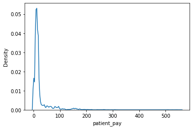
Data is very right skewed. Also, patient_pay is positive only with values of zero, so a hurdle-Gamma model may be appropriate.
import numpy as np
np.sum(pharmacy_train.patient_pay == 0)
869914
How much does pay vary by pharmacy?
plot_data = \
    pharmacy_train \
    .groupby("pharmacy") \
    .aggregate({"patient_pay" : "mean"}) \
    .reset_index() \
    .sort_values("patient_pay")

plt.figure(figsize=(10, 8))
plt.scatter(
    x = "pharmacy",
    y = "patient_pay",
    data = plot_data
)
<matplotlib.collections.PathCollection at 0x2f583f070>
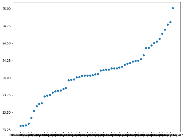
There doesn’t seem to be much variance in pay by location.
How much does pay vary by diagnosis?
plot_data = \
    pharmacy_train \
    .groupby("diagnosis") \
    .aggregate({"patient_pay" : "mean"}) \
    .reset_index() \
    .sort_values("patient_pay")

plt.figure(figsize=(10, 8))
plt.scatter(
    x = "diagnosis",
    y = "patient_pay",
    data = plot_data
)
<matplotlib.collections.PathCollection at 0x2f5981d50>
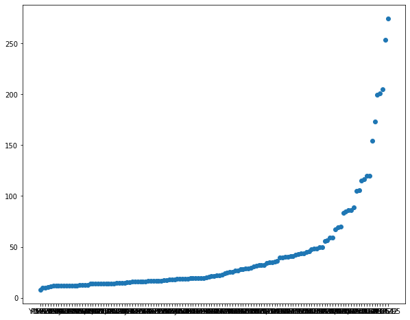
There is substantial variance in pay by the diagnosis type.
How much does pay vary by drug?
plot_data = \
    pharmacy_train \
    .groupby("drug") \
    .aggregate({"patient_pay" : "mean"}) \
    .reset_index() \
    .sort_values("patient_pay")

plt.figure(figsize=(10, 8))
plt.scatter(
    x = "drug",
    y = "patient_pay",
    data = plot_data
)
<matplotlib.collections.PathCollection at 0x2f5b471f0>
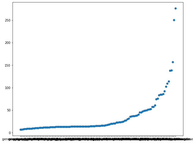
There is also substantial variance in pay by drug type and the plot looks almost identical to the diagnosis plot. This is likely because there is a strong correlation between diagnosis and drug. We will explore that below.
How much does pay vary by insurance plan?
plot_data = \
    pharmacy_train \
    .groupby("bin") \
    .aggregate({"patient_pay" : "mean"}) \
    .reset_index() \
    .sort_values("patient_pay")

plt.figure(figsize=(10, 8))
plt.scatter(
    x = "bin",
    y = "patient_pay",
    data = plot_data
)
<matplotlib.collections.PathCollection at 0x2f5cc4640>
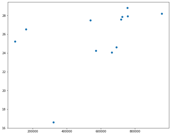
There is a reasonable amount of variance in pay by insurance.
Rejected Claims
sns.catplot(
    x = "rejected",
    kind = "count",
    data = pharmacy_train
)
<seaborn.axisgrid.FacetGrid at 0x2f5cc5e10>
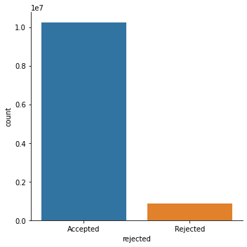
The vast majority of claims were approved.
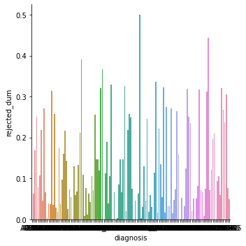
Do approval rates vary by diagnosis?
plot_data = \
    pharmacy_train \
    .assign(rejected_dum = lambda x: np.where(x.rejected == "Rejected", 1, 0)) \
    .groupby("diagnosis") \
    .aggregate({"rejected_dum" : "mean"}) \
    .reset_index()

plt.figure(figsize=(10, 8))
sns.catplot(
    y = "rejected_dum",
    x = "diagnosis",
    kind = "bar",
    data = plot_data.sort_values("rejected_dum")
)
<seaborn.axisgrid.FacetGrid at 0x2f5944b80>


<Figure size 720x576 with 0 Axes>
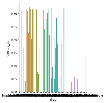
Do approval rates vary by drug type?
plot_data = \
    pharmacy_train \
    .assign(rejected_dum = lambda x: np.where(x.rejected == "Rejected", 1, 0)) \
    .groupby("drug") \
    .aggregate({"rejected_dum" : "mean"}) \
    .reset_index()

plt.figure(figsize=(10, 8))
sns.catplot(
    y = "rejected_dum",
    x = "drug",
    kind = "bar",
    data = plot_data.sort_values("rejected_dum")
)
<seaborn.axisgrid.FacetGrid at 0x30afc1180>


<Figure size 720x576 with 0 Axes>
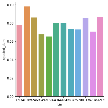
Do approval rates vary by insurance plan?
plot_data = \
    pharmacy_train \
    .assign(rejected_dum = lambda x: np.where(x.rejected == "Rejected", 1, 0)) \
    .groupby("bin") \
    .aggregate({"rejected_dum" : "mean"}) \
    .reset_index()

plt.figure(figsize=(10, 8))
sns.catplot(
    y = "rejected_dum",
    x = "bin",
    kind = "bar",
    data = plot_data.sort_values("rejected_dum")
)
<seaborn.axisgrid.FacetGrid at 0x3b035a8c0>


<Figure size 720x576 with 0 Axes>
Medication Groupings
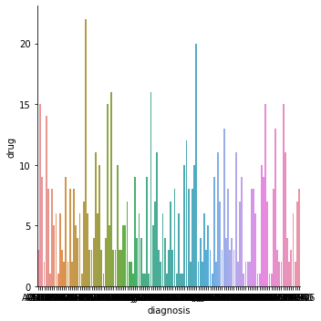
Is there a relationship between diagnosis and drug?
plot_data = \
    pharmacy_train \
    .loc[:, ["diagnosis", "drug"]] \
    .groupby("diagnosis") \
    .nunique() \
    .sort_values("drug") \
    .reset_index()

plt.figure(figsize=(10, 8))
sns.catplot(
    y = "drug",
    x = "diagnosis",
    kind = "bar",
    data = plot_data
)
<seaborn.axisgrid.FacetGrid at 0x30afc07c0>


<Figure size 720x576 with 0 Axes>
Summary of EDA Findings
-
These data are patient transactions that are nested within store and time. The nested structure suggests a multilevel approach and it will be assumed that each row represents a unique patient.
-
Patiant transactions have a substancial variance with diagnosis type, drug type, and insurance type. This indicates that these variables will be important explanatory factors.
-
The majority of claims are approved, and this holds across diagnoses, drug types, and insurance plans.
-
There are some diagnoses that only have one drug option, but the majority have more than one option.