Create train-test split:

set.seed(1)
pharmacy_split <- initial_split(pharmacy_data, prop = 0.8)
pharmacy_train <- training(pharmacy_split)
pharmacy_test <- testing(pharmacy_split)

Examine the training data:

glimpse(pharmacy_train)

## Rows: 11,128,195
## Columns: 13
## $ tx_date      <date> 2022-10-18, 2022-10-11, 2022-01-25, 2022-11-17, 2022-02-…
## $ pharmacy     <fct> Pharmacy #0, Pharmacy #29, Pharmacy #13, Pharmacy #39, Ph…
## $ diagnosis    <fct> I68.27, Z98.86, Z20.23, I38.43, U41.19, K87.68, G99.93, U…
## $ drug         <fct> branded prazinib, branded thiostasteglume, branded flacel…
## $ bin          <fct> 725700, 664344, 691847, 322463, 725700, 664344, 571569, 6…
## $ pcn          <fct> 1UQC, CS8580, 6ZGS97C, 3O71UTS, 1UQC, CS8580, KB38N, NC7E…
## $ group        <fct> NA, NA, NA, NA, NA, NA, 6BYJBW, NA, RS5RB3YA, S2QKZ0OFNWS…
## $ rejected     <lgl> FALSE, FALSE, TRUE, TRUE, FALSE, FALSE, FALSE, FALSE, FAL…
## $ patient_pay  <dbl> 13.39, 20.94, 0.00, 0.00, 13.39, 10.58, 10.84, 17.91, 12.…
## $ claim_status <fct> Approved, Approved, Rejected, Rejected, Approved, Approve…
## $ generic_drug <fct> 0, 0, 0, 0, 0, 1, 0, 0, 0, 0, 0, 0, 1, 0, 0, 0, 1, 1, 1, …
## $ tx_month     <ord> Oct, Oct, Jan, Nov, Feb, Nov, May, May, Dec, Jul, Jul, Oc…
## $ tx_year      <dbl> 2022, 2022, 2022, 2022, 2022, 2022, 2022, 2022, 2022, 202…

# examine the structure of the data
pharmacy_train %>% 
  group_by(pharmacy) %>% 
  summarize(n())

## # A tibble: 58 × 2
##    pharmacy      `n()`
##    <fct>         <int>
##  1 Pharmacy #0  191727
##  2 Pharmacy #1  195563
##  3 Pharmacy #10 201465
##  4 Pharmacy #11 199030
##  5 Pharmacy #12 198913
##  6 Pharmacy #13 175935
##  7 Pharmacy #14 183566
##  8 Pharmacy #15 194972
##  9 Pharmacy #16 196779
## 10 Pharmacy #17 200823
## # … with 48 more rows

pharmacy_train %>% 
  group_by(tx_date, pharmacy) %>% 
  summarize(n())

## `summarise()` has grouped output by 'tx_date'. You can override using the
## `.groups` argument.

## # A tibble: 21,054 × 3
## # Groups:   tx_date [363]
##    tx_date    pharmacy     `n()`
##    <date>     <fct>        <int>
##  1 2022-01-02 Pharmacy #0    107
##  2 2022-01-02 Pharmacy #1    101
##  3 2022-01-02 Pharmacy #10   112
##  4 2022-01-02 Pharmacy #11   103
##  5 2022-01-02 Pharmacy #12   113
##  6 2022-01-02 Pharmacy #13   110
##  7 2022-01-02 Pharmacy #14   114
##  8 2022-01-02 Pharmacy #15   108
##  9 2022-01-02 Pharmacy #16   118
## 10 2022-01-02 Pharmacy #17   108
## # … with 21,044 more rows

Patient transactions are nested within store (pharmacy) and time (tx_date). I will assume that every row represents a unique patient, but the repeated rows of pharmacy and date indicate that it will be important to account for the nested structure of the data. A multilevel model may be useful here.

map_df(pharmacy_train %>% select(pharmacy:tx_year), n_distinct)

## # A tibble: 1 × 12
##   pharmacy diagnosis  drug   bin   pcn group rejected patient_pay claim_status
##      <int>     <int> <int> <int> <int> <int>    <int>       <int>        <int>
## 1       58       133   114    12    49    49        2       20424            2
## # … with 3 more variables: generic_drug <int>, tx_month <int>, tx_year <int>

There are many different types of diagnoses, drugs, and insurance plans in the data. These data are also spread over just one year.

Finally, we check for missing values.

map_df(pharmacy_train %>% select(everything()), ~ sum(is.na(.x)))

## # A tibble: 1 × 13
##   tx_date pharmacy diagnosis  drug   bin     pcn   group rejected patient_pay
##     <int>    <int>     <int> <int> <int>   <int>   <int>    <int>       <int>
## 1       0        0         0     0     0 2902036 3126275        0           0
## # … with 4 more variables: claim_status <int>, generic_drug <int>,
## #   tx_month <int>, tx_year <int>

There are quite a few missing values in the detailed insurance categories of pcn and group.

Copayments by Approval Status

First, we examine patient copayments by their insurance claim status.

ggplot(data = pharmacy_train, aes(x = patient_pay, fill = claim_status,
                                  color = claim_status)) +
  geom_density(adjust = 100) +
  labs(x = "Patient Copayment", y = "Density", fill = "Claim Status",
       color = "Claim Status") +
  ggpubr::theme_pubclean()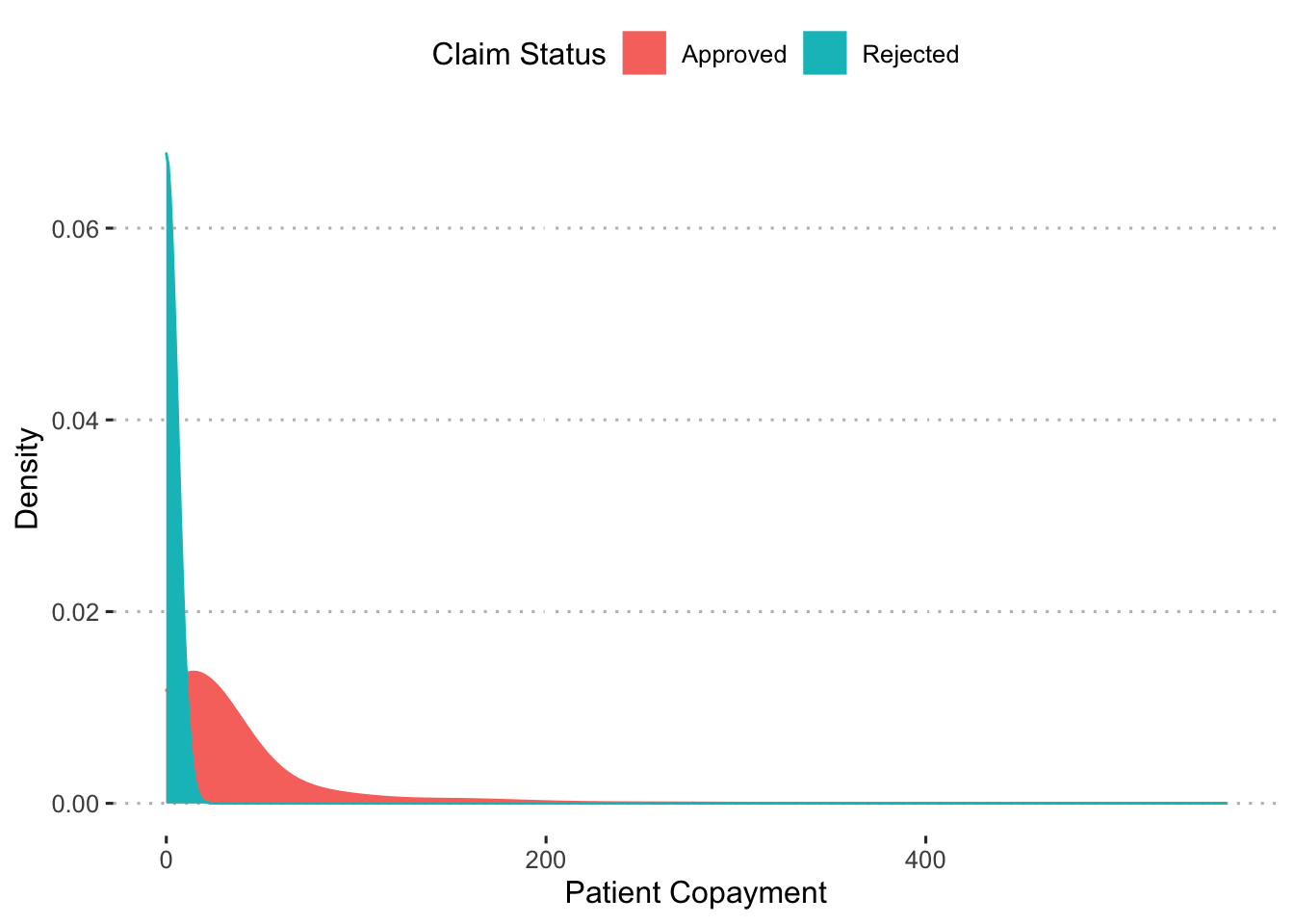

The copayments for patients with rejected claims hover near zero while the copayments for patients with approved claims max out at around 200.

pharmacy_train %>% 
  group_by(rejected) %>% 
  summarize(mean_pay = mean(patient_pay), 
            sd_pay = sd(patient_pay),
            min_pay = min(patient_pay),
            n = n())

## # A tibble: 2 × 5
##   rejected mean_pay sd_pay min_pay        n
##   <lgl>       <dbl>  <dbl>   <dbl>    <int>
## 1 FALSE        26.1   40.5     3.4 10259103
## 2 TRUE          0      0       0     869092

Patients with rejected claims pay nothing and there is no deviation in that amount. Patients with approved claims pay $26 with a standard deviation of $40. Additionally, there are no copayments of zero. This suggests that removing rejected claims from the data may be useful since these observations will provide no predictive benefit.

Copayments Over Time

Is there variation in payments over time? Since our data spans the course of one year, we can look for monthly (or daily) variation.

pharmacy_train %>% 
  filter(claim_status == "Approved") %>% 
  ggplot(aes(x = tx_month, y = log(patient_pay))) +
  geom_boxplot() +
  labs(x = "Transaction Month", 
       y = "Log(Patient Copayment") +
  ggpubr::theme_pubclean()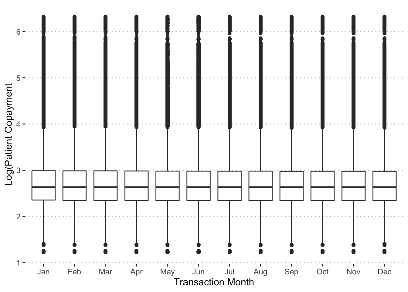

Copayment amounts are very stable over the year. Is there variation within months?

pharmacy_train %>% 
  filter(claim_status == "Approved") %>% 
  ggplot(aes(x = tx_date, y = log(patient_pay), group = tx_date)) +
  geom_boxplot() +
  labs(x = "Transaction Month", 
       y = "Log(Patient Copayment)") +
  scale_x_date(date_labels = "%b-%d", date_breaks = "month") +
  ggpubr::theme_pubclean() +
  theme(axis.text.x = element_text(angle = 45, hjust = 1))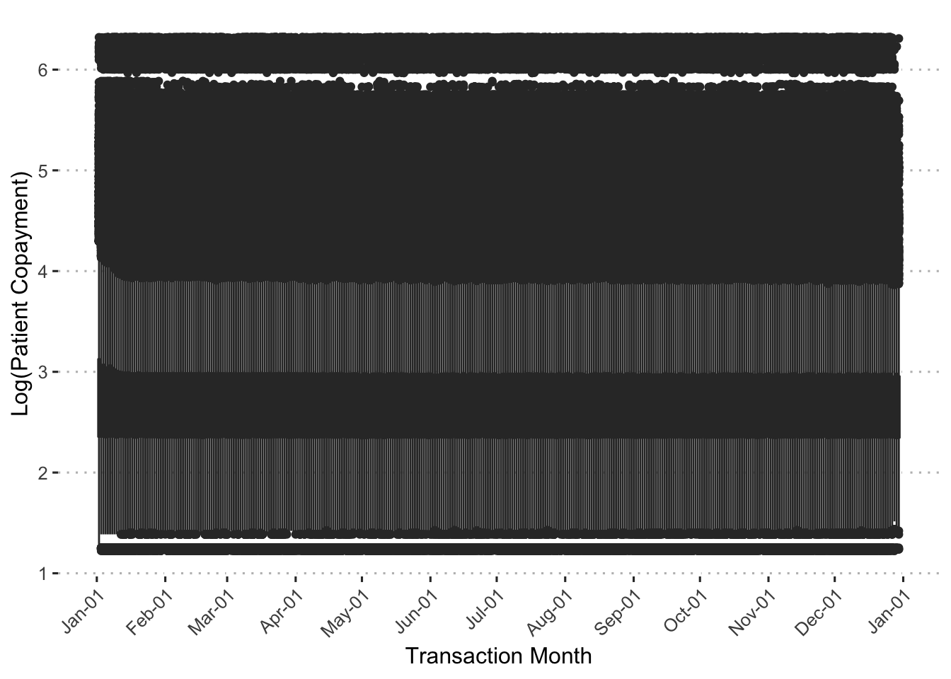

Copayment amounts are very stable within months as well. Overall, there doesn’t seem to be any temporal variation in patient copayments.

Copayments by Location

Next, we examine the level of variation in copayments across pharmacies.

pharmacy_data %>% 
  filter(claim_status == "Approved") %>% 
  ggplot(aes(x = reorder(pharmacy, log(patient_pay)), y = log(patient_pay))) +
  geom_boxplot() +
  scale_y_continuous(breaks = scales::pretty_breaks(n = 8)) +
  labs(x = "Transaction Location", 
       y = "Log(Patient Copayment)") +
  ggpubr::theme_pubclean() +
  theme(axis.text.x = element_text(angle = 45, hjust = 1))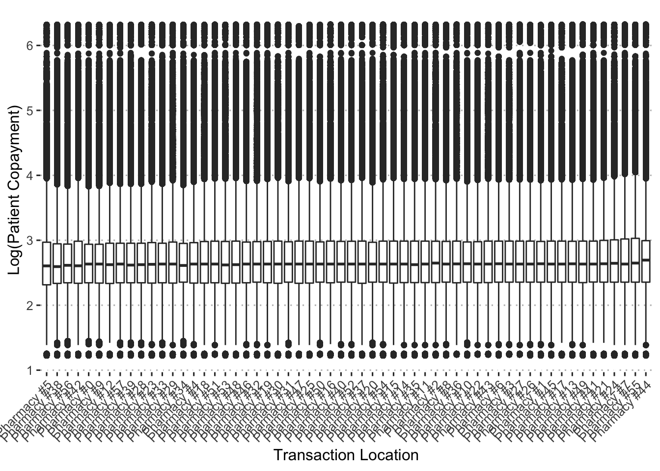

Copayments are consistent across pharmacy locations.

Copayments by Insurance Plan

Before examining how copayments vary across insurance plans, we first need to get a sense of how many different insurance plans and subcategories there are.

pharmacy_train %>% 
  filter(claim_status == "Approved") %>% 
  group_by(bin) %>% 
  summarize(n_pcn = n_distinct(pcn),
            n_group = n_distinct(group)) %>% 
  pivot_longer(cols = c(n_pcn, n_group), names_to = "group", 
               values_to = "count") %>% 
  ggplot(aes(x = reorder(bin, count), y = count, fill = group)) +
  geom_col(position = position_dodge()) +
  labs(x = "Insurance Plan",
       y = "Distinct Groups",
       fill = "Subcategory") +
  ggpubr::theme_pubclean()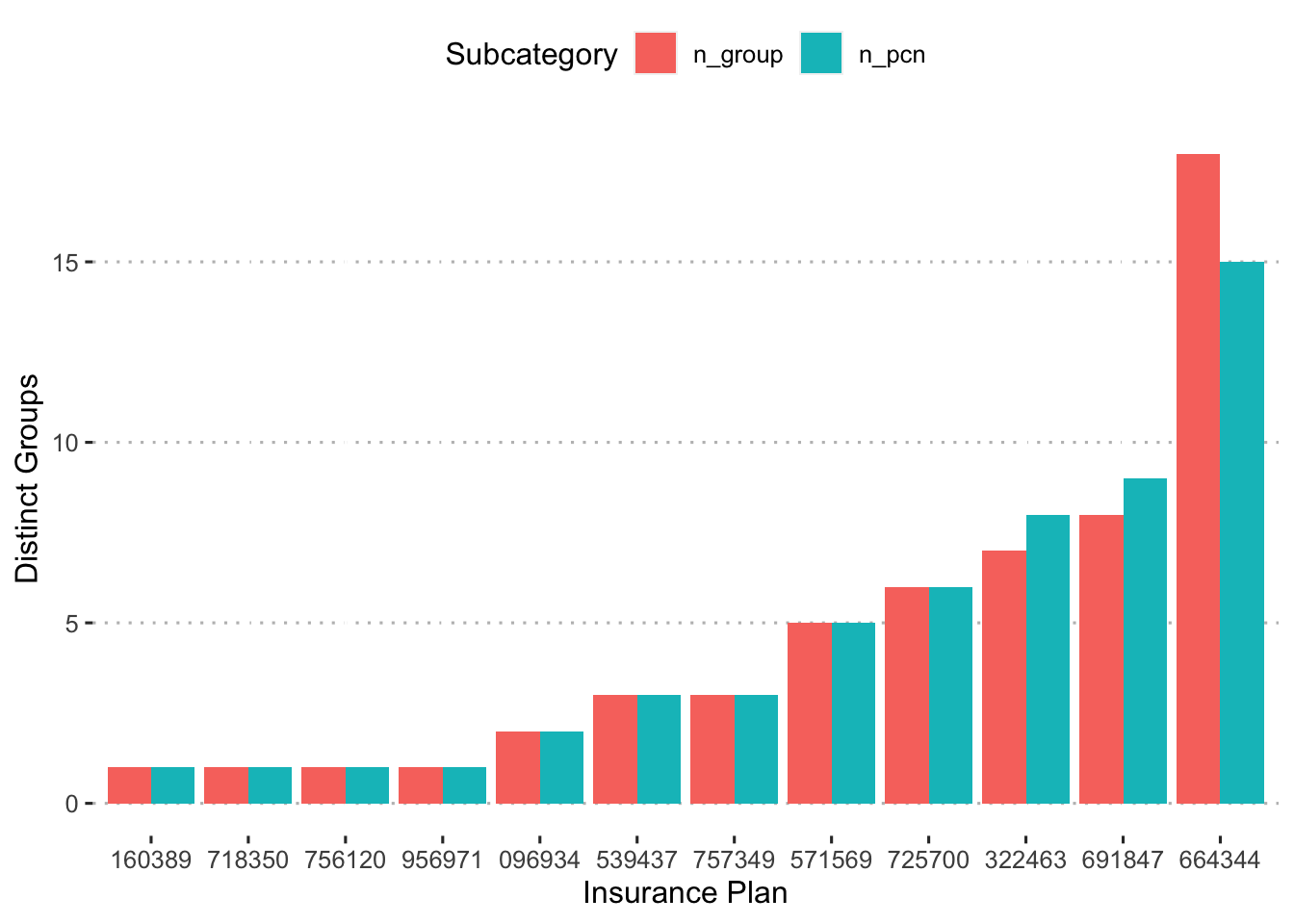

There are 12 total insurance plans and the smallest number of insurance options for any insurance plan is one. For example, plan 956971 offers one pcn and one group. On the other hand, 096934 offers two different pcns with two different groups each for a total of four options.

pharmacy_train %>% group_by(bin, pcn) %>% distinct(group)

## # A tibble: 63 × 3
## # Groups:   bin, pcn [55]
##    bin    pcn     group        
##    <fct>  <fct>   <fct>        
##  1 725700 1UQC    <NA>         
##  2 664344 CS8580  <NA>         
##  3 691847 6ZGS97C <NA>         
##  4 322463 3O71UTS <NA>         
##  5 571569 KB38N   6BYJBW       
##  6 691847 NC7EN   <NA>         
##  7 160389 RB7UU   RS5RB3YA     
##  8 725700 9C5MOR3 S2QKZ0OFNWS6X
##  9 725700 BZ22Z2  ZOYKF0N5NEO  
## 10 718350 J5DT8   IX6P0        
## # … with 53 more rows

This shows that each group is unique to each pcn. Additionally, there doesn’t seem to be multiple groups per pcn.

How much variation in copayments across insurance plans?

pharmacy_train %>% 
  filter(claim_status == "Approved") %>% 
  ggplot(aes(x = reorder(bin, log(patient_pay)), y = log(patient_pay))) +
  geom_boxplot() +
  labs(x = "Insurance Plan", y = "Log(Patient Copayment)") +
  ggpubr::theme_pubclean()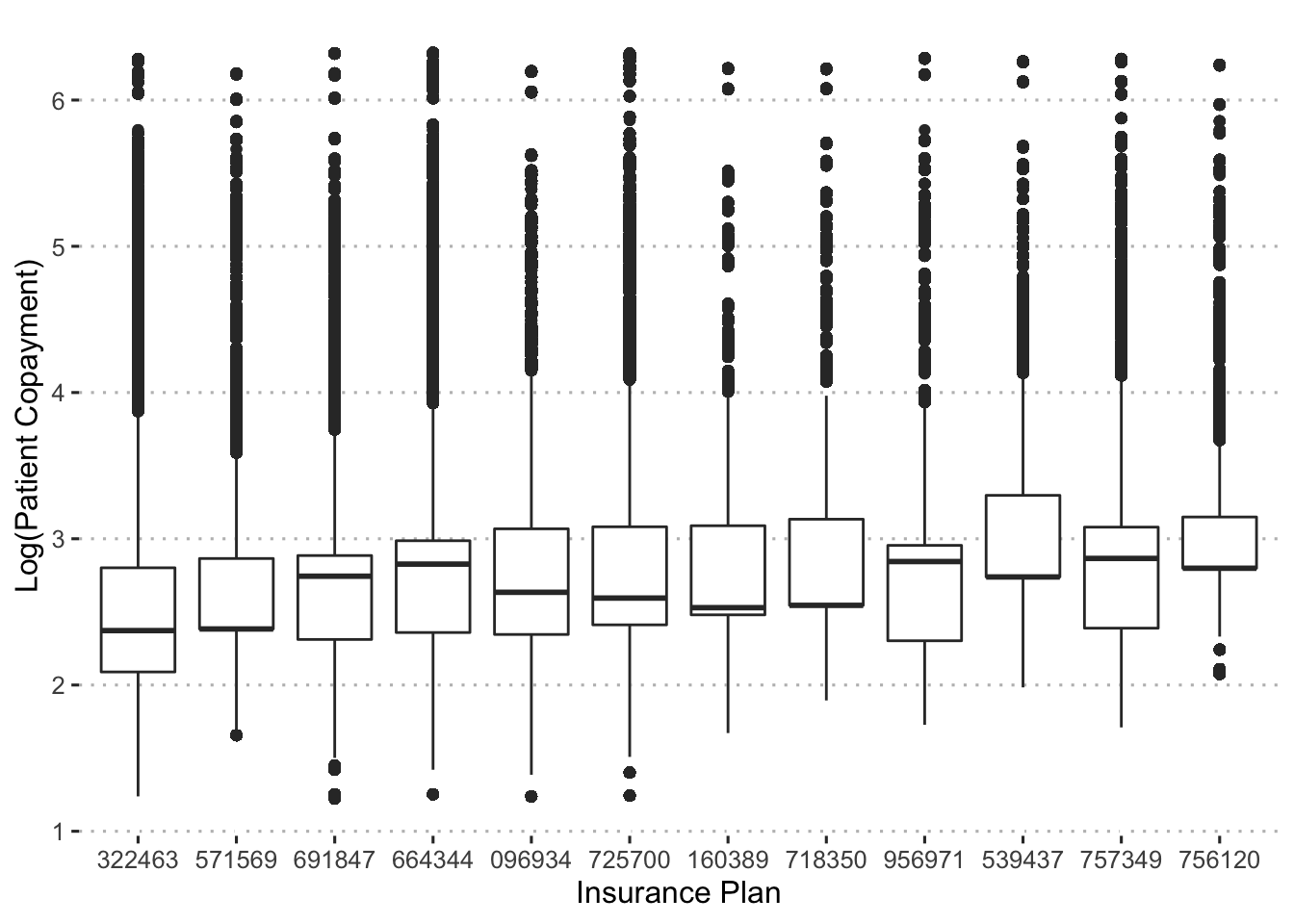

There is a small amount of variance in patient copayments by insurance plan with the mean values ranging from about $12 to $16.

Finally, let’s examine how much variation in copayments there is within insurance plans (across pcns and groups).

pharmacy_train %>% 
  filter(claim_status == "Approved") %>% 
  ggplot(aes(x = reorder(pcn, log(patient_pay)),
             y = log(patient_pay), fill = group)) +
  geom_boxplot() +
  facet_wrap(~ bin, scales = "free") +
  labs(x = "PCN", y = "Log(Patient Copayment)", 
       subtitle = "Colors indicate different subcategories of pcn.") +
  ggpubr::theme_pubclean() +
  theme(legend.position = "none")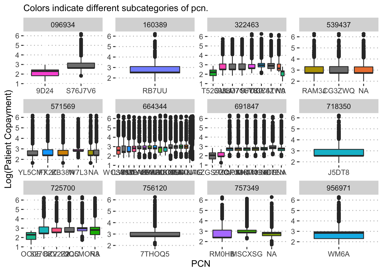

There is also a good amount of variance in copayments by insurance plan subcategory.

Copayments by Diagnosis

Here we examine how copayments vary by diagnosis. As noted above, there are 133 diagnoses in the data. Each diagnosis starts with a letter and in total there are 25 different leading letters.

Using these leading letters, we’ll examine the variation in copayments across diagnosis group:

pharmacy_train %>% 
  filter(claim_status == "Approved") %>% 
  mutate(diagnosis_collapsed = str_sub(diagnosis, start = 1L, end = 1L)) %>% 
  ggplot(aes(x = reorder(diagnosis_collapsed, log(patient_pay)), y = log(patient_pay))) +
  geom_boxplot() +
  labs(x = "Broad Diagnosis Category",
       y = "Log(Patient Copayment)") +
  ggpubr::theme_pubclean()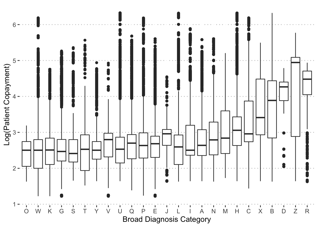

Diagnosis category “R” has the highest average copayment, while category “O” has the lowest. Overall, there is quite a bit of variation across categories. Now let’s examine how much variation there is in copayments within each diagnosis group.

pharmacy_train %>% 
  filter(claim_status == "Approved") %>% 
  mutate(diagnosis_collapsed = str_sub(diagnosis, start = 1L, end = 1L)) %>% 
  select(patient_pay, diagnosis, diagnosis_collapsed) %>% 
  ggplot(aes(x = reorder(diagnosis, log(patient_pay)), y = log(patient_pay))) +
  geom_boxplot() +
  facet_wrap(~ diagnosis_collapsed, scales = "free") +
  labs(x = "Diagnosis Category",
       y = "Log(Patient Copayment)") +
  ggpubr::theme_pubclean()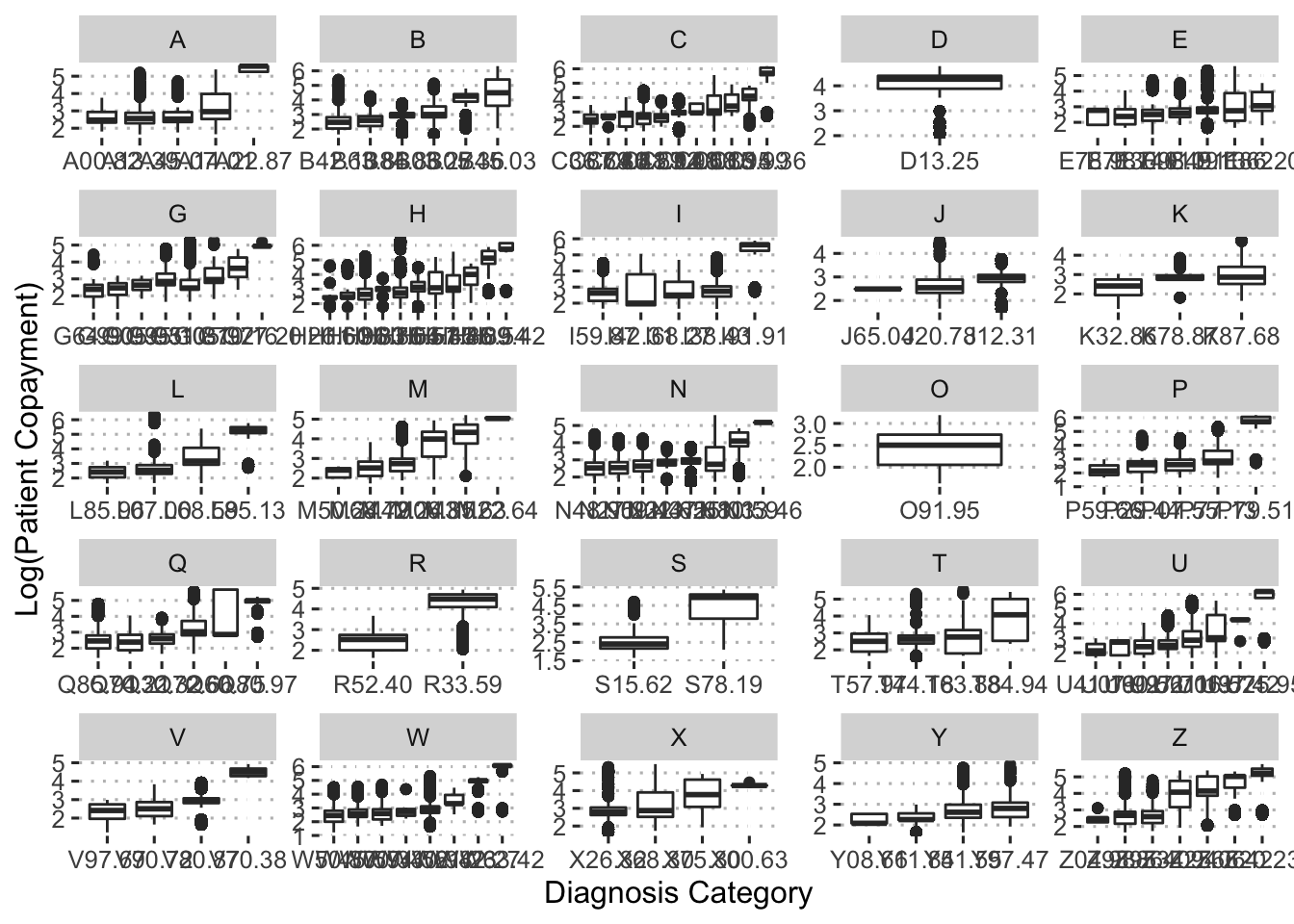

This plot shows that there is also a substantial amount of variance in copayments within each diagnosis group.

Copayments by Drug

In this section, we examine how copayments vary with the drug prescribed. There are 114 unique drugs in the data.

pharmacy_train %>% 
  filter(claim_status == "Approved") %>% 
  janitor::tabyl(generic_drug)

##  generic_drug       n   percent
##             0 6141769 0.5986653
##             1 4117334 0.4013347

Of these 114 drugs, 40% are generic and about 60% are branded.

pharmacy_train %>% 
  filter(claim_status == "Approved") %>% 
  ggplot(aes(x = generic_drug, y = log(patient_pay))) +
  geom_boxplot() +
  labs(x = "Drug Type",
       y = "Log(Patient Copayment)") +
  scale_x_discrete(labels = c("Branded", "Generic")) +
  ggpubr::theme_pubclean()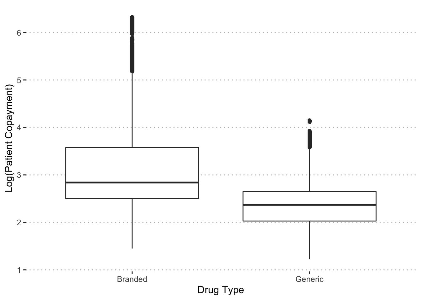

Perhaps as expected, generic drugs are associated with lower copayments. Alternatively, we can compare the mean copayments for branded and generic drugs within each drug group.

pharmacy_train %>% 
  filter(claim_status == "Approved") %>%
  mutate(drug_alt = str_replace(drug, "generic|branded", ""),
         drug_alt = str_trim(drug_alt, side = "both")) %>% 
  ggplot(aes(x = generic_drug, y = log(patient_pay))) +
  geom_boxplot() +
  facet_wrap(~ drug_alt, scales = "free") +
  labs(x = "Drug Type",
       y = "Log(Patient Copayment)") +
  scale_x_discrete(labels = c("Branded", "Generic")) +
  ggpubr::theme_pubclean()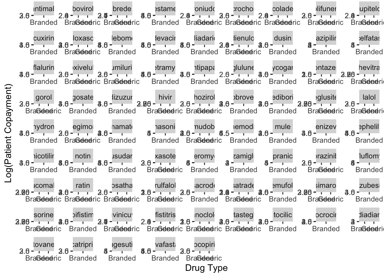

There are some drugs that don’t have a generic option, but in every case the generics have lower copayments.

Now we evaluate how copayments vary by generic status across diagnoses.

pharmacy_train %>% 
  filter(claim_status == "Approved") %>% 
  mutate(diagnosis_collapsed = str_sub(diagnosis, start = 1L, end = 1L)) %>%
  ggplot(aes(x = generic_drug, y = log(patient_pay))) +
  geom_boxplot() +
  facet_wrap(~ diagnosis_collapsed, scales = "free") +
  labs(x = "Drug Type",
       y = "Log(Patient Copayment)") +
  scale_x_discrete(labels = c("Branded", "Generic")) +
  ggpubr::theme_pubclean()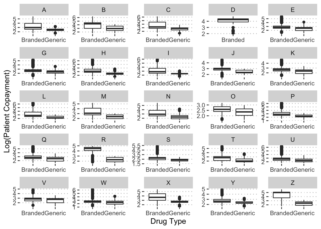

There is only one diagnosis without a generic drug option and across the board, generic drugs have lower copayments.

We can also examine the copayments for each drug within each broad diagnosis category.

pharmacy_train %>% 
  filter(claim_status == "Approved") %>% 
  mutate(diagnosis_collapsed = str_sub(diagnosis, start = 1L, end = 1L)) %>%
  ggplot(aes(x = reorder(drug, log(patient_pay)), y = log(patient_pay))) +
  geom_boxplot() +
  facet_wrap(~ diagnosis_collapsed, scales = "free") +
  labs(x = "Drug Type",
       y = "Log(Patient Copayment)") +
  ggpubr::theme_pubclean() +
  theme(axis.text.x = element_text(angle = 45, hjust = 1))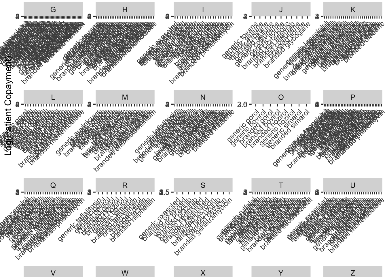

Finally, we can also compare the copayments for each drug within each insurance plan.

pharmacy_train %>% 
  filter(claim_status == "Approved") %>%
  mutate(drug_alt = str_replace(drug, "generic|branded", ""),
         drug_alt = str_trim(drug_alt, side = "both")) %>% 
  ggplot(aes(x = reorder(bin, log(patient_pay)), y = log(patient_pay), 
             fill = generic_drug)) +
  geom_boxplot() +
  facet_wrap(~ drug_alt, scales = "free") +
  labs(x = "Drug Type",
       y = "Log(Patient Copayment)",
       fill = "Drug Type") +
  scale_fill_discrete(label = c("Branded", "Generic")) +
  ggpubr::theme_pubclean() +
  theme(axis.text.x = element_text(angle = 45, hjust = 1))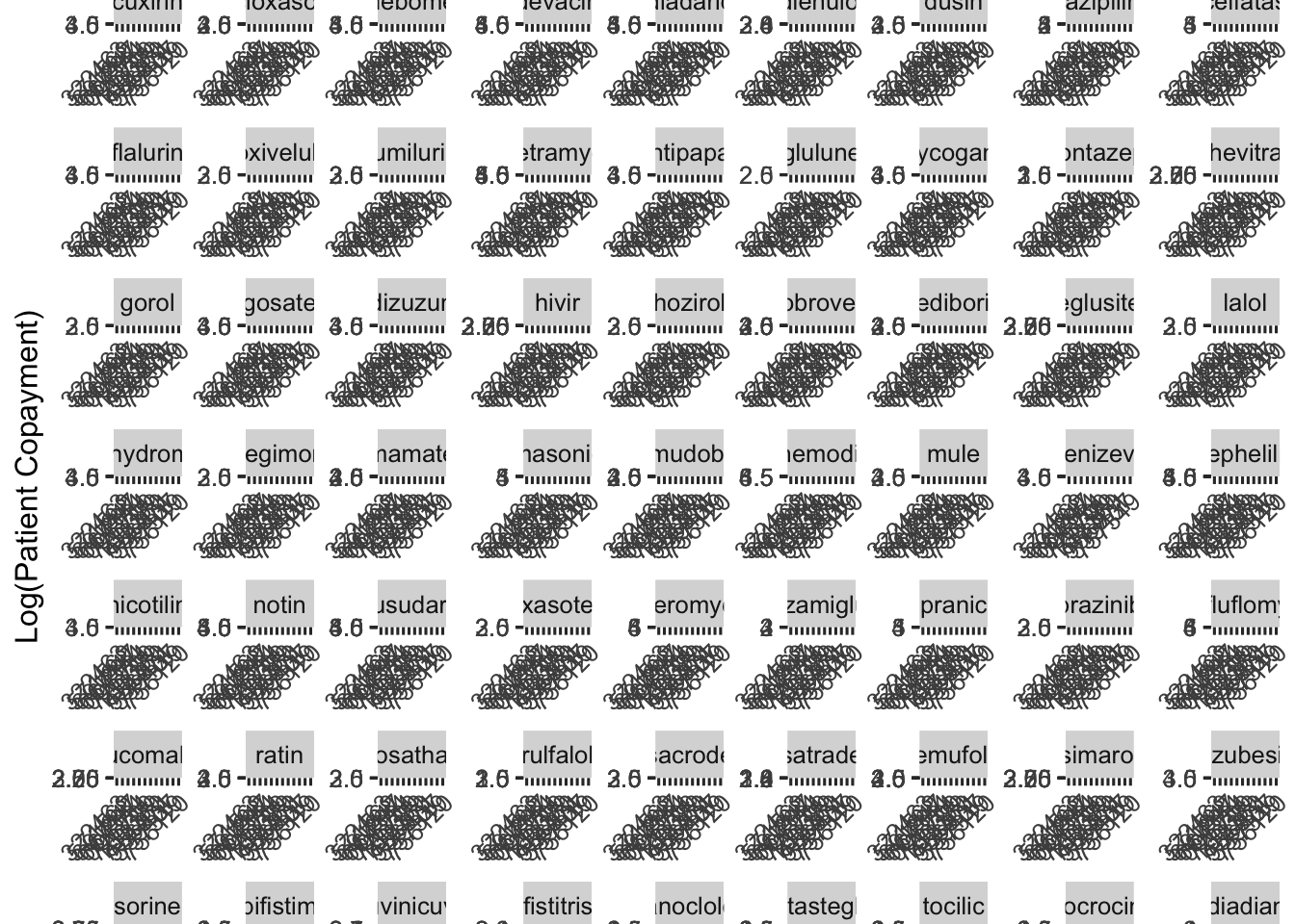

Here we see that there is a significant degree of variation in drug copayments across insurance plans.

Summary of Patient Copayment EDA

The following patterns have emerged after exploring patient copayments:

1. The majority of claims are approved but there were no approved claims that had a $0 copayment. In addition, all rejected claims had a $0 copayment with no variation.
2. There is little to no variation in copayments over the course of the year.
3. There is little to no variation in copayments across pharmacy locations.
4. There is a small amount of variation in copayments across broad insurance plans and that variance increases with more detailed levels of insurance plan groups and pcns.
5. There is a substantial amount of variance in copayments across diagnosis type.
6. Branded drugs have a slight majority over generics, and are always associated with higher copays. There is also a large amount of variance in copays across insurance plans for a given diagnosis.

These findings indicated that broad and detailed insurance plan, drug type, and diagnosis will all be important predictors of patient copayments.