Insurance Claim Data Science Project: Data Analysis

With the data cleaned, and an understanding of the relationships between variables, I now build predictive models to understand patient copayments and insurance claim approvals.

These models are primarily built with the tidymodels package.

knitr::opts_chunk$set(cache = TRUE)
library(pacman)
p_load(tidyverse, tidymodels, lubridate, baguette, finetune, embed)
tidymodels_prefer()

Import the Data and Clean

I start my analysis by importing the data and performing some basic cleaning.

pharmacy_data_raw <- read_csv("pharmacy_tx.csv", num_threads = 4)

## Rows: 13910244 Columns: 9
## ── Column specification ────────────────────────────────────────────────────────
## Delimiter: ","
## chr  (6): pharmacy, diagnosis, drug, bin, pcn, group
## dbl  (1): patient_pay
## lgl  (1): rejected
## date (1): tx_date
## 
## ℹ Use `spec()` to retrieve the full column specification for this data.
## ℹ Specify the column types or set `show_col_types = FALSE` to quiet this message.

# recode variables
pharmacy_data <- 
  pharmacy_data_raw %>% 
  mutate(claim_status = factor(rejected,
                               levels = c("FALSE", "TRUE"),
                               labels = c("Approved", "Rejected"))) %>% 
  mutate(across(where(is.character), as.factor),
         across(where(is.logical), as.factor))

# drop rejected claims
pharmacy_data <- 
  pharmacy_data %>% 
  filter(claim_status == "Approved") %>% 
  drop_na()

# the data set is too large for my local machine to run models on!
set.seed(1)
pharmacy_data <- 
  pharmacy_data %>% 
  sample_n(size = 10000)

Create Train Test Split

Next, I split the data into training and testing partitions and create folds for cross-validation. I choose to create 5 folds that are repeated 3 times each.

# train-test split
set.seed(2)
pharmacy_split <- initial_split(pharmacy_data, prop = 0.8)
pharmacy_train <- training(pharmacy_split)
pharmacy_test <- testing(pharmacy_split)

# cross-validation folds
folds <- vfold_cv(pharmacy_train, v = 5, repeats = 3)

Objective I: Predict Patient Copayments

To accomplish this objective, I fit a series of prediction models to predict a patient’s copayment based on the variables in the data.

Model Building

Model Specifications

With the data prepped, I now create the model specifications complete with several preprocessing steps. These steps include:

Extracting the month of the transaction to serve as a feature
Dropping the transaction date from the estimation data
Log transforming the response variable
Grouping infrequently occurring diagnoses into an “Other Diagnoses” category
Creating dummy variables for each categorical variable
Removing variables with no variation

Finally, for the linear models I also include:

The interactions of all insurance plans with all drugs
The interactions of all diagnoses with all drugs

# Linear model without interactions
linear_recipe <- 
  recipe(patient_pay ~ ., data = pharmacy_train) %>% 
  step_date(tx_date, features = "month") %>% 
  step_rm(tx_date, group, pcn) %>%
  step_log(patient_pay) %>% 
  step_other(diagnosis, threshold = 20, other = "Other Diagnoses") %>% 
  step_dummy(all_nominal_predictors()) %>% 
  step_zv(all_predictors())

# Linear model with interactions
linear_int_recipe <- 
  recipe(patient_pay ~ ., data = pharmacy_train) %>% 
  step_date(tx_date, features = "month") %>% 
  step_rm(tx_date, group, pcn) %>%
  step_log(patient_pay) %>% 
  step_other(diagnosis, threshold = 20, other = "Other Diagnoses") %>% 
  step_dummy(all_nominal_predictors()) %>% 
  step_interact(~ starts_with("bin"):starts_with("drug")) %>%
  step_interact(~ starts_with("diagnosis"):starts_with("drug")) %>%
  step_zv(all_predictors())

# no dummy recipe
no_dum_recipe <- 
  recipe(patient_pay ~ ., data = pharmacy_train) %>% 
  step_date(tx_date, features = "month") %>% 
  step_rm(tx_date, group, pcn) %>%
  step_log(patient_pay) %>% 
  step_zv(all_predictors())

Models

To patient copayments, I will use the following models:

Regularized linear regression
K-nearest neighbors
Boosted tree
Random forest
Support vector machine

# linear models ---------------------------------------------------------------
linear_model <- 
  linear_reg(penalty = tune(), mixture = tune()) %>% 
  set_engine("glmnet")

knn_reg_model <- 
  nearest_neighbor(neighbors = tune(), dist_power = tune(), 
                   weight_func = tune()) %>% 
  set_engine("kknn") %>% 
  set_mode("regression")

# decision tree models --------------------------------------------------------
xgboost_reg_model <- 
   boost_tree(tree_depth = tune(), learn_rate = tune(), loss_reduction = tune(),
              min_n = tune(), sample_size = tune(), trees = tune()) %>% 
   set_engine("xgboost") %>% 
   set_mode("regression")

rf_reg_model <- 
  rand_forest(min_n = tune(), trees = 1000) %>% 
  set_engine("ranger") %>% 
  set_mode("regression")

# support vector machines -----------------------------------------------------
svm_reg_model <- 
   svm_rbf(cost = tune(), rbf_sigma = tune()) %>% 
   set_engine("kernlab") %>% 
   set_mode("regression")

Model Workflow Prep

# linear models with and without interactions ---------------------------------
linear_reg_wflows <- 
  workflow_set(
    preproc = list(no_int = linear_recipe, int = linear_int_recipe),
    models = list(linear_reg = linear_model, knn = knn_reg_model),
    cross = TRUE
  )

# tree models -----------------------------------------------------------------
rf_reg_wflow <-
  workflow_set(
    preproc = list(base = no_dum_recipe),
    models = list(rf = rf_reg_model)
  )

xgboost_reg_wflow <-
  workflow_set(
    preproc = list(no_int = linear_recipe),
    models = list(xgboost = xgboost_reg_model)
  )

# support vector machine ------------------------------------------------------
svm_reg_wflow <-
  workflow_set(
    preproc = list(no_int = linear_recipe),
    models = list(svm = svm_reg_model)
  )

# combine all tuning workflows ------------------------------------------------
all_reg_workflows <- 
  bind_rows(linear_reg_wflows, rf_reg_wflow, xgboost_reg_wflow, svm_reg_wflow)

Model Tuning and Fitting

Model Testing

Before fitting the models to the full training set, I first estimate them on a much smaller random sample of data from the training set to identify any model specification errors. This way I can more efficiently ensure that the models will run on the full data without issue.

I use Bayesian optimization to tune the model parameters.

# test models on a smaller sample to identify errors
set.seed(2)
model_testing_data <- 
  pharmacy_train %>% 
  sample_n(size = 1000)

# cross-validation folds
test_folds <- vfold_cv(model_testing_data, v = 3)

bayes_control <- control_bayes(no_improve = 20, verbose = TRUE,
                               parallel_over = "everything")

# initialize parallelization
library(doMC)
registerDoMC(cores = 4)

# testing linear models with and without interactions -------------------------
linear_reg_results <- 
  linear_reg_wflows %>% 
  workflow_map(
    seed = 1, 
    fn = "tune_bayes",
    resamples = test_folds,
    initial = 5, 
    iter = 2,
    control = bayes_control,
    verbose = TRUE
  )

# testing tree models ---------------------------------------------------------
rf_reg_results <- 
  rf_reg_wflow %>% 
  workflow_map(
    seed = 1, 
    fn = "tune_bayes",
    resamples = test_folds,
    initial = 5, 
    iter = 2,
    control = bayes_control,
    verbose = TRUE
  )

xgboost_reg_results <- 
  xgboost_reg_wflow %>% 
  workflow_map(
    seed = 1, 
    fn = "tune_bayes",
    resamples = test_folds,
    initial = 10, 
    iter = 2,
    control = bayes_control,
    verbose = TRUE
  )

# testing support vector machine ----------------------------------------------
svm_reg_results <- 
  svm_reg_wflow %>% 
  workflow_map(
    seed = 1, 
    fn = "tune_bayes",
    resamples = test_folds,
    initial = 5, 
    iter = 2,
    control = bayes_control,
    verbose = TRUE
  )

Full Model Fitting

Now I fit and tune the models to the full cross-validation folds.

all_reg_results <- 
  all_reg_workflows %>% 
  workflow_map(
    seed = 1, 
    fn = "tune_bayes",
    resamples = folds,
    initial = 15, 
    iter = 10,
    control = bayes_control,
    verbose = TRUE
  )

# save fitted workflow
save(all_reg_results, file = "all_reg_results.Rda")

Model Evaluation

With the models fit, we now explore the best results of each model to compare their performance.

all_reg_results %>% 
  rank_results() %>% 
  filter(.metric == "rmse") %>% 
  group_by(model) %>% 
  slice_min(rank) %>% 
  select(model, .config, rmse = mean, rank) %>% 
  arrange(rank)

## # A tibble: 5 × 4
## # Groups:   model [5]
##   model            .config                rmse  rank
##   <chr>            <chr>                 <dbl> <int>
## 1 linear_reg       Preprocessor1_Model12 0.317     1
## 2 boost_tree       Preprocessor1_Model01 0.338    23
## 3 nearest_neighbor Preprocessor1_Model02 0.343    24
## 4 svm_rbf          Iter10                0.349    29
## 5 rand_forest      Iter1                 0.408    86

The linear regression with interaction terms had the lowest RMSE, followed by the boosted tree. These results will also vary depending on the seletecd optimization precedure.

We can also visually compare the best model specifications:

# plot results
autoplot(all_reg_results, rank_metric = "rmse", metric = c("rmse", "rsq"), 
         select_best = TRUE) +
  geom_text(aes(y = mean - 0.008, label = wflow_id, angle = 90, hjust = 1)) +
  labs(y = "Metric") +
  theme_classic() +
  theme(legend.position = "none")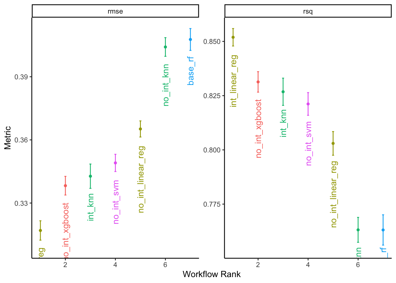

Model Finalization

Let’s examine the chosen parameters of the best performing model.

best_results <- 
  all_reg_results %>% 
  extract_workflow_set_result("int_linear_reg") %>% 
  select_best(metric = "rmse")

best_results

## # A tibble: 1 × 3
##    penalty mixture .config              
##      <dbl>   <dbl> <chr>                
## 1 0.000458   0.761 Preprocessor1_Model12

Now, we can use the tuned parameter values to finalize our model and fit the model to the full training set.

final_reg_wflow <- 
  all_reg_results %>% 
  extract_workflow("int_linear_reg") %>% 
  finalize_workflow(best_results)

final_reg_wflow

## ══ Workflow ════════════════════════════════════════════════════════════════════
## Preprocessor: Recipe
## Model: linear_reg()
## 
## ── Preprocessor ────────────────────────────────────────────────────────────────
## 8 Recipe Steps
## 
## • step_date()
## • step_rm()
## • step_log()
## • step_other()
## • step_dummy()
## • step_interact()
## • step_interact()
## • step_zv()
## 
## ── Model ───────────────────────────────────────────────────────────────────────
## Linear Regression Model Specification (regression)
## 
## Main Arguments:
##   penalty = 0.00045776023577091
##   mixture = 0.760780365400327
## 
## Computational engine: glmnet

We execute the final fit with last_fit() which fits the final model on the full training data and evaluates the finalized model on the testing data.

final_reg_fit <- 
  final_wflow %>% 
  last_fit(pharmacy_split)

save(final_reg_fit, file = "final_reg_fit.Rda")

Finalized Predictions

With the final model chosen, we can examine the performance metrics on the testing data:

collect_metrics(final_reg_fit)

## # A tibble: 2 × 4
##   .metric .estimator .estimate .config             
##   <chr>   <chr>          <dbl> <chr>               
## 1 rmse    standard       0.305 Preprocessor1_Model1
## 2 rsq     standard       0.855 Preprocessor1_Model1

We’ll also examine the model’s predictions plotted against the actual values:

augment(final_reg_fit) %>% 
  ggplot(aes(x = patient_pay, y = exp(.pred))) +
  geom_point(alpha = 0.5) +
  geom_abline(lty = 2) +
  coord_obs_pred() +
  labs(x = "Observed Patient Pay", y = "Predicted Patient Pay") +
  theme_minimal()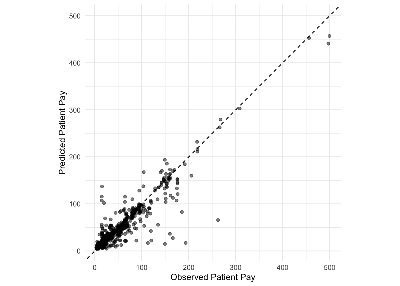

Points above the line indicate over-predictions while points below the line indicate under-predictions.

Now we examine the predicted copayments by diagnosis category:

augment(final_reg_fit) %>% 
  mutate(diagnosis_collapsed = str_sub(diagnosis, start = 1L, end = 1L)) %>% 
  group_by(diagnosis_collapsed) %>% 
  summarize(obs_mean = mean(patient_pay),
            pred_mean = mean(exp(.pred))) %>% 
  ggplot() +
  geom_point(aes(x = reorder(diagnosis_collapsed, obs_mean), y = obs_mean), 
             shape = 1, size = 4, alpha = 1.5) +
  geom_point(aes(x = reorder(diagnosis_collapsed, pred_mean), y = pred_mean), 
             shape = 19, size = 4, color = "red", alpha = 0.7) +
  labs(x = "Broad Diagnosis Category",
       y = "Patient Copayment",
       subtitle = "Open circles represent the observed copayment and the red circles show the predicted copayment.") +
  scale_y_continuous(labels = dollar_format(),
                     breaks = pretty_breaks(n = 8)) +
  ggpubr::theme_pubclean()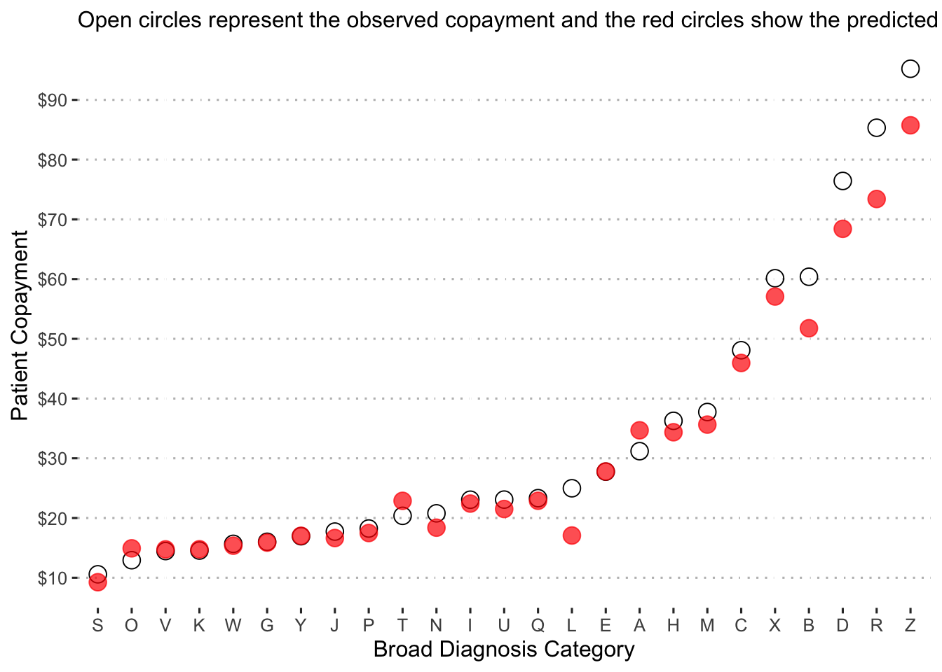

Diagnosis “S” is predicted to have the lowest copayment on average at just over $10, while diagnosis “Z” is predicted to have the highest with a value of about $95.

We can also visualize this figure broken down by the drug prescribed:

augment(final_reg_fit) %>% 
  mutate(diagnosis_collapsed = str_sub(diagnosis, start = 1L, end = 1L),
         generic_drug = ifelse(str_detect(drug, "generic"), 1, 0),
         generic_drug = as_factor(generic_drug)) %>% 
  group_by(diagnosis_collapsed, generic_drug) %>% 
  summarize(obs_mean = mean(patient_pay),
            pred_mean = mean(exp(.pred))) %>% 
  ggplot() +
  geom_point(aes(x = reorder(generic_drug, obs_mean), y = obs_mean), 
             shape = 1, size = 4, alpha = 1.5) +
  geom_point(aes(x = reorder(generic_drug, pred_mean), y = pred_mean), 
             shape = 19, size = 4, color = "red", alpha = 0.7) +
  facet_wrap( ~ diagnosis_collapsed, scales = "free") +
  labs(x = "Broad Diagnosis Category",
       y = "Patient Copayment",
       subtitle = "Open circles represent the observed copayment and the red circles show the predicted copayment.") +
  scale_x_discrete(labels = c("Generic", "Branded")) +
  scale_y_continuous(labels = dollar_format(),
                     breaks = pretty_breaks(n = 5)) +
  ggpubr::theme_pubclean()

## `summarise()` has grouped output by 'diagnosis_collapsed'. You can override
## using the `.groups` argument.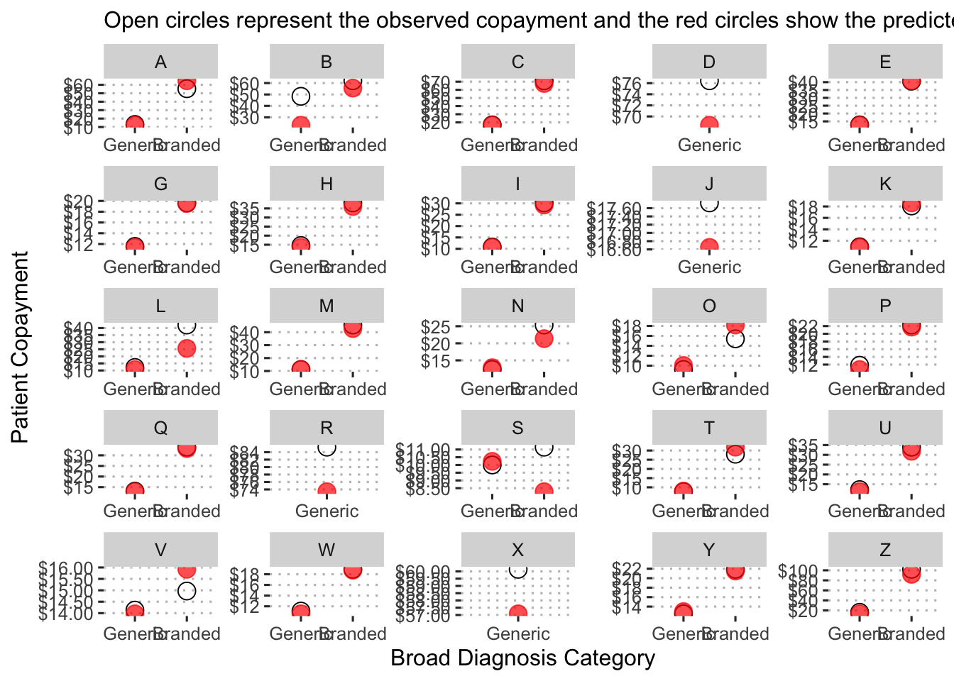

Here we can see the predicted mean copayments by drug type (branded or generic) for each broad diagnosis category.

Finally, we can examine the predicted copayment by insurance plan for each drug.

augment(final_reg_fit) %>% 
  mutate(generic_drug = ifelse(str_detect(drug, "generic"), 1, 0),
         generic_drug = as_factor(generic_drug)) %>% 
  group_by(bin, pcn, generic_drug) %>% 
  summarize(obs_mean = mean(patient_pay),
            pred_mean = mean(exp(.pred))) %>% 
  ggplot() +
  geom_point(aes(x = reorder(pcn, obs_mean), y = obs_mean, color = generic_drug), 
             shape = 1, size = 4, alpha = 1.5) +
  geom_point(aes(x = reorder(pcn, pred_mean), y = pred_mean, color = generic_drug), 
             shape = 19, size = 4, alpha = 0.7) +
  facet_wrap( ~ bin, scales = "free", ncol = 3) +
  labs(x = "Detailed Insurance Plan",
       y = "Patient Copayment",
       color = "Drug Type",
       subtitle = "Open circles represent the observed copayment and the red circles show the predicted copayment.") +
  scale_color_discrete(labels = c("Branded", "Generic")) +
  scale_y_continuous(labels = dollar_format(),
                     breaks = pretty_breaks(n = 5)) +
  ggpubr::theme_pubclean()

## `summarise()` has grouped output by 'bin', 'pcn'. You can override using the
## `.groups` argument.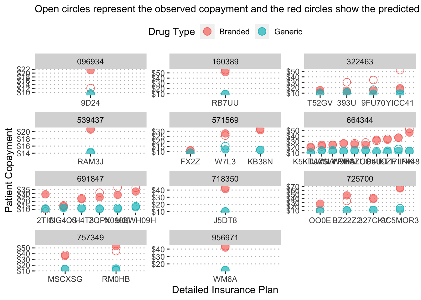

This figure shows the predicted copayment for branded and generic drugs under each insurance plan by pcn to provide a sense of how much a drug would cost under a detailed insurance plan.

We could also examine the predicted copayment for specific drugs across insurance plans:

augment(final_reg_fit) %>% 
  mutate(generic_drug = ifelse(str_detect(drug, "generic"), 1, 0),
         generic_drug = as_factor(generic_drug),
         drug_alt = str_replace(drug, "generic|branded", ""),
         drug_alt = str_trim(drug_alt, side = "both")) %>% 
  group_by(bin, drug_alt, generic_drug) %>% 
  summarize(obs_mean = mean(patient_pay),
            pred_mean = mean(exp(.pred))) %>%
  ggplot() +
  geom_point(aes(x = reorder(bin, obs_mean), y = obs_mean, color = generic_drug), 
             shape = 1, size = 4, alpha = 1.5) +
  geom_point(aes(x = reorder(bin, pred_mean), y = pred_mean, color = generic_drug), 
             shape = 19, size = 4, alpha = 0.7) +
  facet_wrap(~ drug_alt, scales = "free") +
  labs(x = "Insurance Plan",
       y = "Patient Copayment",
       color = "Drug Type",
       subtitle = "Open circles represent the observed copayment and the red circles show the predicted copayment.") +
  scale_fill_discrete(label = c("Branded", "Generic")) +
  scale_color_discrete(labels = c("Branded", "Generic")) +
  scale_y_continuous(labels = dollar_format(),
                     breaks = pretty_breaks(n = 5)) +
  ggpubr::theme_pubclean() +
  theme(axis.text.x = element_text(angle = 45, hjust = 1))

## `summarise()` has grouped output by 'bin', 'drug_alt'. You can override using
## the `.groups` argument.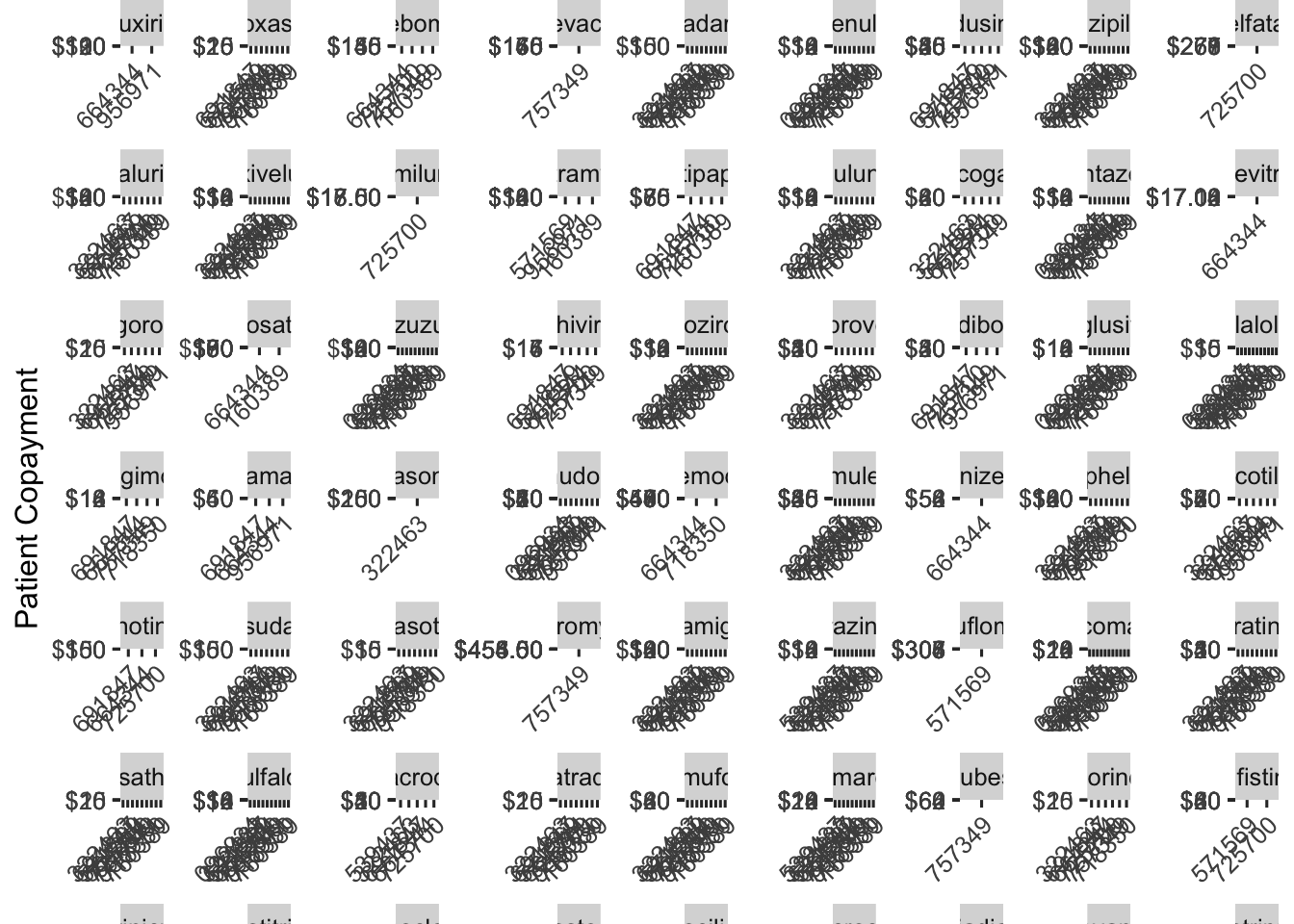

This plot shows predicted copayment of a given drug across insurance plans. To make it easier to digest, we could select a single drug to examine. Hivir, for example:

augment(final_reg_fit) %>% 
  mutate(generic_drug = ifelse(str_detect(drug, "generic"), 1, 0),
         generic_drug = as_factor(generic_drug),
         drug_alt = str_replace(drug, "generic|branded", ""),
         drug_alt = str_trim(drug_alt, side = "both")) %>% 
  group_by(bin, drug_alt, generic_drug) %>% 
  summarize(obs_mean = mean(patient_pay),
            pred_mean = mean(exp(.pred))) %>%
  filter(drug_alt == "hivir") %>% 
  ggplot() +
  geom_point(aes(x = reorder(bin, obs_mean), y = obs_mean, color = generic_drug), 
             shape = 1, size = 4, alpha = 1.5) +
  geom_point(aes(x = reorder(bin, pred_mean), y = pred_mean, color = generic_drug), 
             shape = 19, size = 4, alpha = 0.7) +
  facet_wrap(~ drug_alt, scales = "free") +
  labs(x = "Insurance Plan",
       y = "Patient Copayment",
       color = "Drug Type",
       subtitle = "Open circles represent the observed copayment and the red circles show the predicted copayment.") +
  scale_fill_discrete(label = c("Branded", "Generic")) +
  scale_color_discrete(labels = c("Branded", "Generic")) +
  scale_y_continuous(labels = dollar_format(),
                     breaks = pretty_breaks(n = 5)) +
  ggpubr::theme_pubclean() +
  theme(axis.text.x = element_text(angle = 45, hjust = 1))

## `summarise()` has grouped output by 'bin', 'drug_alt'. You can override using
## the `.groups` argument.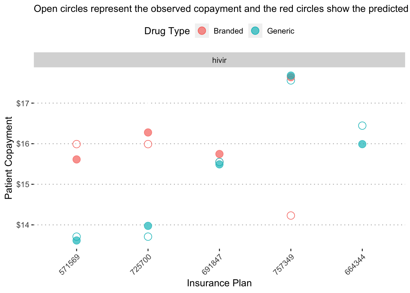

On insurance plan “571569”, the a generic form of the drug “hivir” is predicted to have a copayment of a little less than $14 while its branded alternative is predicted to have a copayment close to $16.

Objective II: Predict the formulary status of the medication on each insurance plan

To accomplish this objective, we will use classification models to estimate the probability of an insurance claim being rejected or not. Then, we group these predicted probabilities into three groups to capture their formulary status according to rejected, non-preferred, and preferred:

Predicted probabilities between $[0, 0.5)$ are grouped into the rejected group
Predicted probabilities between $[0.5, 0.75)$ are grouped into the non-preferred group
Predicted probabilities between $[0.75, 1.0]$ are grouped into the preferred group

With these groups, we can further determine whether each drug is a generic, preferred non-generic, non-preferred non-generic, etc.

To start, the rejected claims need to be added back to the data set and I will create a new train-test split and validation folds.

pharmacy_data <- 
  pharmacy_data_raw %>% 
  mutate(claim_status = factor(rejected,
                               levels = c("FALSE", "TRUE"),
                               labels = c("Approved", "Rejected"))) %>% 
  mutate(across(where(is.character), as.factor),
         across(where(is.logical), as.factor))

# the data set is too large for my local machine to run models on!
set.seed(1)
pharmacy_data <- 
  pharmacy_data %>% 
  sample_n(size = 10000)

# train-test split
set.seed(2)
pharmacy_split <- initial_split(pharmacy_data, prop = 0.8, strata = claim_status)
pharmacy_train <- training(pharmacy_split)
pharmacy_test <- testing(pharmacy_split)

# cross-validation folds
folds <- vfold_cv(pharmacy_train, v = 5, repeats = 3, strata = claim_status)

Model Building

Model Specifications

For the classification models, I use the following preprocessing steps:

Extracting the month of the transaction to serve as a feature
Dropping the transaction date from the estimation data
Log transforming the response variable
Grouping infrequently occurring diagnoses into an “Other Diagnoses” category
Creating dummy variables for each categorical variable
Removing variables with no variation

Finally, for the linear models I also include:

The interactions of all insurance plans with all drugs
The interactions of all diagnoses with all drugs

# Linear model without interactions
linear_recipe <- 
  recipe(claim_status ~ ., data = pharmacy_train) %>% 
  step_date(tx_date, features = "month") %>%
  step_rm(tx_date, patient_pay, rejected, group, pcn) %>%
  step_other(diagnosis, threshold = 20, other = "Other Diagnoses") %>% 
  step_dummy(all_nominal_predictors()) %>% 
  step_novel(all_nominal_predictors()) %>%
  step_zv(all_predictors())

# Linear model with interactions
linear_int_recipe <- 
  recipe(claim_status ~ ., data = pharmacy_train) %>% 
  step_date(tx_date, features = "month") %>% 
  step_rm(tx_date, patient_pay, rejected, group, pcn) %>%
  step_other(diagnosis, threshold = 20, other = "Other Diagnoses") %>% 
  step_dummy(all_nominal_predictors()) %>% 
  step_novel(all_nominal_predictors()) %>%
  step_interact(~ starts_with("bin"):starts_with("drug")) %>%
  step_interact(~ starts_with("diagnosis"):starts_with("drug")) %>%
  step_zv(all_predictors())

# no dummy recipe
no_dum_recipe <- 
  recipe(claim_status ~ ., data = pharmacy_train) %>% 
  step_date(tx_date, features = "month") %>% 
  step_rm(tx_date, patient_pay, rejected, group, pcn) %>%
  step_zv(all_predictors())

Models

To classify claim status, I will use the following models:

K-nearest neighbors
Linear discriminant analysis
Regularized Binomial regression (with a Logit link function)
Naive Bayes
Boosted tree
Random forest
Support vector machine

# load packages for engines
p_load(discrim, mda, brulee, klaR)

# k-nearest neighbors ---------------------------------------------------------
knn_c_model <- 
  nearest_neighbor(neighbors = tune(), dist_power = tune(), 
                   weight_func = tune()) %>% 
  set_engine("kknn") %>% 
  set_mode("classification")

# linear discriminant analysis ------------------------------------------------
lda_model <- 
  discrim_linear(penalty = tune()) %>% 
  set_engine("mda") %>% 
  set_mode("classification")

# binomial regression ---------------------------------------------------------
binom_model <- 
  logistic_reg(penalty = tune(), mixture = tune()) %>% 
  set_engine("glmnet") %>% 
  set_mode("classification")

# naive bayes -----------------------------------------------------------------
nb_model <- 
  naive_Bayes(smoothness = tune()) %>% 
  set_engine("klaR") %>% 
  set_mode("classification")

# random forest ---------------------------------------------------------------
rf_c_model <- 
  rand_forest(mtry = tune(), min_n = tune(), trees = 1000) %>% 
  set_engine("ranger", importance = "impurity") %>% 
  set_mode("classification")

# xgboost ---------------------------------------------------------------------
xgboost_c_model <- 
  boost_tree(tree_depth = tune(), learn_rate = tune(), loss_reduction = tune(),
              min_n = tune(), sample_size = tune(), trees = tune()) %>% 
   set_engine("xgboost") %>% 
   set_mode("classification")

# support vector machine ------------------------------------------------------
svm_c_model <- 
   svm_rbf(cost = tune(), rbf_sigma = tune()) %>% 
   set_engine("kernlab") %>% 
   set_mode("classification")

Model Workflow Prep

# linear models with and without interactions ---------------------------------
linear_c_wflows <- 
  workflow_set(
    preproc = list(no_int = linear_recipe, int = linear_int_recipe),
    models = list(knn_c = knn_c_model, lda = lda_model, binom = binom_model,
                  nb = nb_model),
    cross = TRUE
  )

# tree models -----------------------------------------------------------------
rf_c_wflow <-
  workflow_set(
    preproc = list(base = no_dum_recipe),
    models = list(rf = rf_c_model)
  )

xgboost_c_wflow <-
  workflow_set(
    preproc = list(no_int = linear_recipe),
    models = list(xgboost_c = xgboost_c_model)
  )

# support vector machine ------------------------------------------------------
svm_c_wflow <-
  workflow_set(
    preproc = list(linear = linear_recipe),
    models = list(svm_c = svm_c_model)
  )

# combine all tuning workflows ------------------------------------------------
all_c_workflows <- 
  bind_rows(linear_c_wflows, rf_c_wflow, xgboost_c_wflow, svm_c_wflow)

Model Tuning and Fitting

Model Testing

As before, I fitting the classification models on a much smaller random sample of data from the training set to identify any model specification errors.

# test models on a smaller sample to identify errors
set.seed(2)
model_testing_data <- 
  pharmacy_train %>% 
  sample_n(size = 1000)

# cross-validation folds
test_folds <- vfold_cv(model_testing_data, v = 2, strata = claim_status)

grid_ctrl <- 
  control_grid(
    save_pred = FALSE, 
    save_workflow = FALSE,
    parallel_over = "everything"
  )

# initialize parallelization
library(doMC)
registerDoMC(cores = 4)

# testing linear models with and without interactions -------------------------
linear_c_results <- 
  linear_c_wflows %>% 
  workflow_map(
    seed = 1, 
    resamples = test_folds,
    grid = 2, 
    control = grid_ctrl,
    verbose = TRUE
  )

# testing tree models ---------------------------------------------------------
rf_c_results <- 
  rf_c_wflow %>% 
  workflow_map(
    seed = 1, 
    resamples = test_folds,
    grid = 2, 
    control = grid_ctrl,
    verbose = TRUE
  )

xgboost_c_results <- 
  xgboost_c_wflow %>% 
  workflow_map(
    seed = 1, 
    resamples = test_folds,
    grid = 2, 
    control = grid_ctrl,
    verbose = TRUE
  )

# testing support vector machine ----------------------------------------------
svm_c_results <- 
  svm_c_wflow %>% 
  workflow_map(
    seed = 1, 
    resamples = test_folds,
    grid = 2, 
    control = grid_ctrl,
    verbose = TRUE
  )

Full Model Fitting

Now I fit and tune the models to the full cross-validation folds.

all_c_results <- 
  all_c_workflows %>% 
  workflow_map(
    seed = 1, 
    resamples = folds,
    grid = 5, 
    control = grid_ctrl,
    verbose = TRUE
  )

# save fitted workflow
save(all_c_results, file = "all_c_results_wflows.Rda")

Model Evaluation

With the models fit, we now explore the best results of each model to compare their performance.

all_c_results %>% 
  rank_results() %>% 
  filter(.metric == "roc_auc") %>% 
  group_by(model) %>% 
  slice_min(rank) %>% 
  #select(model, .config, mean, rank) %>% 
  arrange(rank)

## # A tibble: 7 × 9
## # Groups:   model [7]
##   wflow_id         .config  .metric  mean std_err     n preprocessor model  rank
##   <chr>            <chr>    <chr>   <dbl>   <dbl> <int> <chr>        <chr> <int>
## 1 no_int_binom     Preproc… roc_auc 0.873 0.00337    15 recipe       logi…     1
## 2 no_int_lda       Preproc… roc_auc 0.868 0.00505    15 recipe       disc…     5
## 3 base_rf          Preproc… roc_auc 0.865 0.00327    15 recipe       rand…    10
## 4 int_knn_c        Preproc… roc_auc 0.850 0.00397    15 recipe       near…    15
## 5 no_int_xgboost_c Preproc… roc_auc 0.832 0.00477    15 recipe       boos…    17
## 6 linear_svm_c     Preproc… roc_auc 0.828 0.00304    15 recipe       svm_…    20
## 7 no_int_nb        Preproc… roc_auc 0.5   0          15 recipe       naiv…    46

The regularized binomial regression model with a logit link function and no interaction terms performed best according to the ROC score.

# plot results
autoplot(all_c_results, rank_metric = "roc_auc", select_best = TRUE) +
  geom_text(aes(y = mean - 0.01, label = wflow_id, angle = 90, hjust = 1)) +
  labs(y = "Metric") +
  theme_classic() +
  theme(legend.position = "none")

## Warning: Removed 1 rows containing missing values (geom_point).

## Warning: Removed 1 rows containing missing values (geom_text).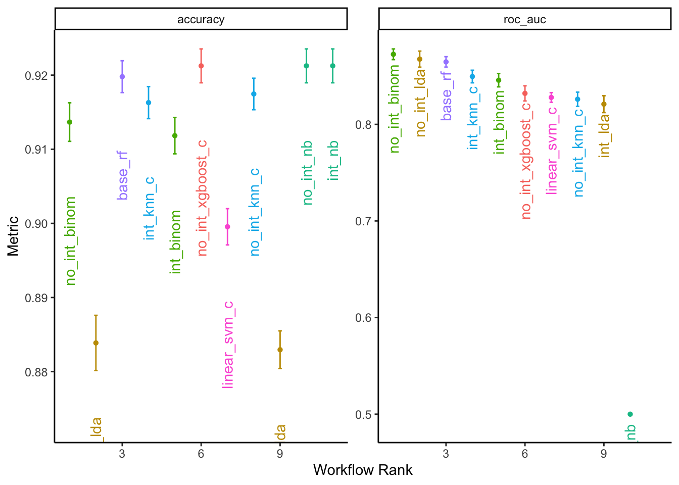

Model Finalization

Let’s examine the chosen parameters of the best performing model.

best_results <- 
  all_c_results %>% 
  extract_workflow_set_result("no_int_binom") %>% 
  select_best(metric = "roc_auc")

best_results

## # A tibble: 1 × 3
##        penalty mixture .config             
##          <dbl>   <dbl> <chr>               
## 1 0.0000000402   0.238 Preprocessor1_Model1

Now, we can use the tuned parameter values to finalize our model and fit the model to the full training set.

final_c_wflow <- 
  all_c_results %>% 
  extract_workflow("no_int_binom") %>% 
  finalize_workflow(best_results)

final_c_wflow

## ══ Workflow ════════════════════════════════════════════════════════════════════
## Preprocessor: Recipe
## Model: logistic_reg()
## 
## ── Preprocessor ────────────────────────────────────────────────────────────────
## 6 Recipe Steps
## 
## • step_date()
## • step_rm()
## • step_other()
## • step_dummy()
## • step_novel()
## • step_zv()
## 
## ── Model ───────────────────────────────────────────────────────────────────────
## Logistic Regression Model Specification (classification)
## 
## Main Arguments:
##   penalty = 4.01885407883291e-08
##   mixture = 0.238281848281622
## 
## Computational engine: glmnet

We execute the final fit with last_fit() which fits the final model on the full training data and evaluates the finalized model on the testing data.

final_c_fit <- 
  final_c_wflow %>% 
  last_fit(pharmacy_split)

save(final_c_fit, file = "final_c_fit.Rda")

Finalized Predictions

With the final model chosen, we can examine some performance metrics on the testing data:

collect_metrics(final_c_fit)

## # A tibble: 2 × 4
##   .metric  .estimator .estimate .config             
##   <chr>    <chr>          <dbl> <chr>               
## 1 accuracy binary         0.920 Preprocessor1_Model1
## 2 roc_auc  binary         0.874 Preprocessor1_Model1

augment(final_c_fit) %>% 
  f_meas(truth = claim_status, estimate = .pred_class)

## # A tibble: 1 × 3
##   .metric .estimator .estimate
##   <chr>   <chr>          <dbl>
## 1 f_meas  binary         0.958

augment(final_c_fit) %>% 
  mcc(truth = claim_status, estimate = .pred_class)

## # A tibble: 1 × 3
##   .metric .estimator .estimate
##   <chr>   <chr>          <dbl>
## 1 mcc     binary        0.0994

We can also visualize ROC and confusion matricies:

augment(final_c_fit) %>% 
  conf_mat(truth = claim_status, estimate = .pred_class) %>% 
  autoplot()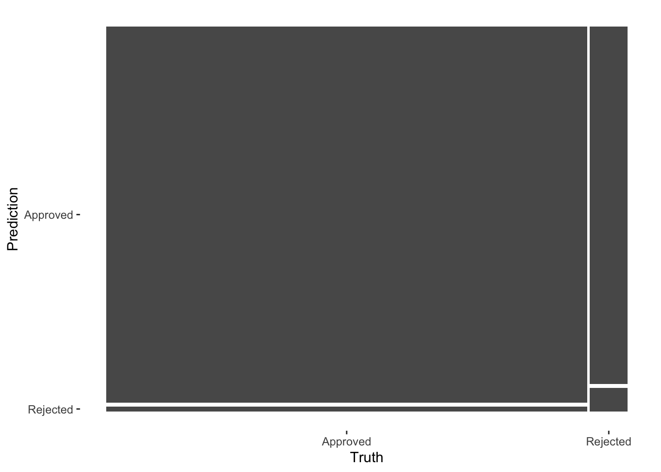

augment(final_c_fit) %>% 
  roc_curve(truth = claim_status, estimate = .pred_Approved) %>% 
  autoplot()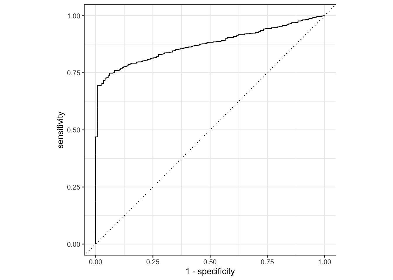

The model does make reasonably accurate predictions, but it struggles because of so few zeros in the data.

Now let’s put some of the model’s predictions into context. First, we’ll examine the approval rates across insurance plan.

augment(final_c_fit) %>% 
  group_by(bin) %>% 
  summarize(.pred_Approved = mean(.pred_Approved)) %>% 
  ggplot() +
  geom_point(aes(x = reorder(bin, .pred_Approved), y = .pred_Approved),
             shape = 19, size = 4, color = "red", alpha = 0.7) +
  labs(x = "Insurance Plan", y = "Predicted Approval Rate") +
  coord_cartesian(ylim = c(0.9, 1)) +
  scale_y_continuous(labels = percent_format(), breaks = pretty_breaks(4)) +
  ggpubr::theme_pubclean()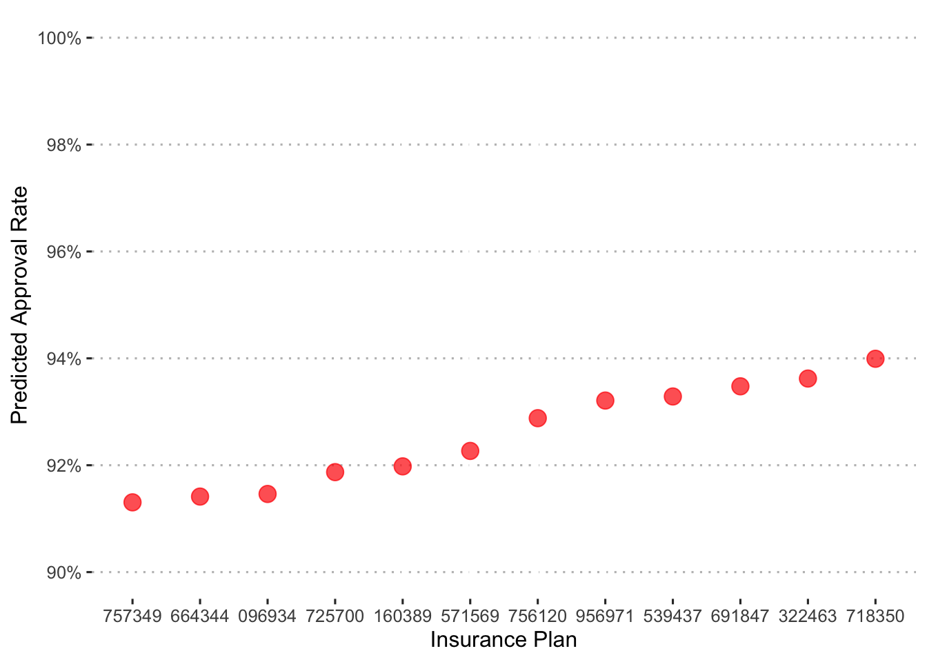

In general, approvals are high with only a little over a 2 point spread across plans.

Let’s see how these approaval rates differ depending on drug type.

augment(final_c_fit) %>% 
  mutate(generic_drug = ifelse(str_detect(drug, "generic"), 1, 0),
         generic_drug = as_factor(generic_drug)) %>% 
  group_by(bin, generic_drug) %>% 
  summarize(.pred_Approved = mean(.pred_Approved)) %>%
  ggplot() +
  geom_point(aes(x = reorder(bin, .pred_Approved), y = .pred_Approved, 
                 color = generic_drug), 
             shape = 19, size = 4, alpha = 0.7) +
  labs(x = "Insurance Plan", y = "Predicted Approval Rate",
       color = "Drug Type") +
  coord_cartesian(ylim = c(0.8, 1)) +
  scale_y_continuous(labels = percent_format(), breaks = pretty_breaks(6)) +
  scale_color_discrete(labels = c("Branded", "Generic")) +
  ggpubr::theme_pubclean()

## `summarise()` has grouped output by 'bin'. You can override using the `.groups`
## argument.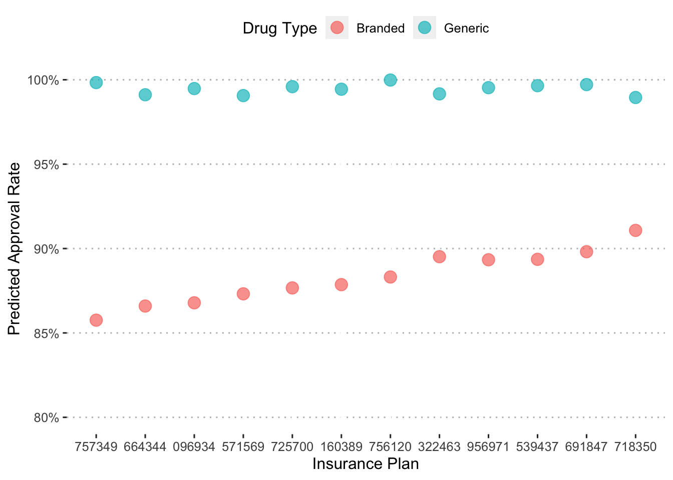

Across insurance plans, branded drugs have much lower approval rates than generics.

But what about the approval rates among specific drugs across insurance plans?

augment(final_c_fit) %>% 
  mutate(generic_drug = ifelse(str_detect(drug, "generic"), 1, 0),
         generic_drug = as_factor(generic_drug),
         drug_alt = str_replace(drug, "generic|branded", ""),
         drug_alt = str_trim(drug_alt, side = "both")) %>% 
  group_by(bin, generic_drug, drug_alt) %>% 
  summarize(.pred_Approved = mean(.pred_Approved)) %>%
  ggplot() +
  geom_point(aes(x = reorder(bin, .pred_Approved), y = .pred_Approved, 
                 color = generic_drug), 
             shape = 19, size = 4, alpha = 0.7) +
  facet_wrap(~ drug_alt, scales = "free") +
  labs(x = "Insurance Plan", y = "Predicted Approval Rate",
       color = "Drug Type") +
  scale_y_continuous(labels = percent_format(), breaks = pretty_breaks(4)) +
  scale_color_discrete(labels = c("Branded", "Generic")) +
  ggpubr::theme_pubclean() +
  theme(axis.text.x = element_text(angle = 45, hjust = 1))

## `summarise()` has grouped output by 'bin', 'generic_drug'. You can override
## using the `.groups` argument.

To more easily understand this plot, we’ll again zoom in on the drug Hivir.

augment(final_c_fit) %>% 
  mutate(generic_drug = ifelse(str_detect(drug, "generic"), 1, 0),
         generic_drug = as_factor(generic_drug),
         drug_alt = str_replace(drug, "generic|branded", ""),
         drug_alt = str_trim(drug_alt, side = "both")) %>% 
  filter(drug_alt == "hivir") %>% 
  group_by(bin, generic_drug, drug_alt) %>% 
  summarize(.pred_Approved = mean(.pred_Approved)) %>%
  ggplot() +
  geom_point(aes(x = reorder(bin, .pred_Approved), y = .pred_Approved, 
                 color = generic_drug), 
             shape = 19, size = 4, alpha = 0.7) +
  labs(x = "Insurance Plan", y = "Predicted Approval Rate",
       color = "Drug Type") +
  scale_y_continuous(labels = percent_format(), breaks = pretty_breaks(6)) +
  scale_color_discrete(labels = c("Branded", "Generic")) +
  ggpubr::theme_pubclean() +
  theme(axis.text.x = element_text(angle = 45, hjust = 1))

## `summarise()` has grouped output by 'bin', 'generic_drug'. You can override
## using the `.groups` argument.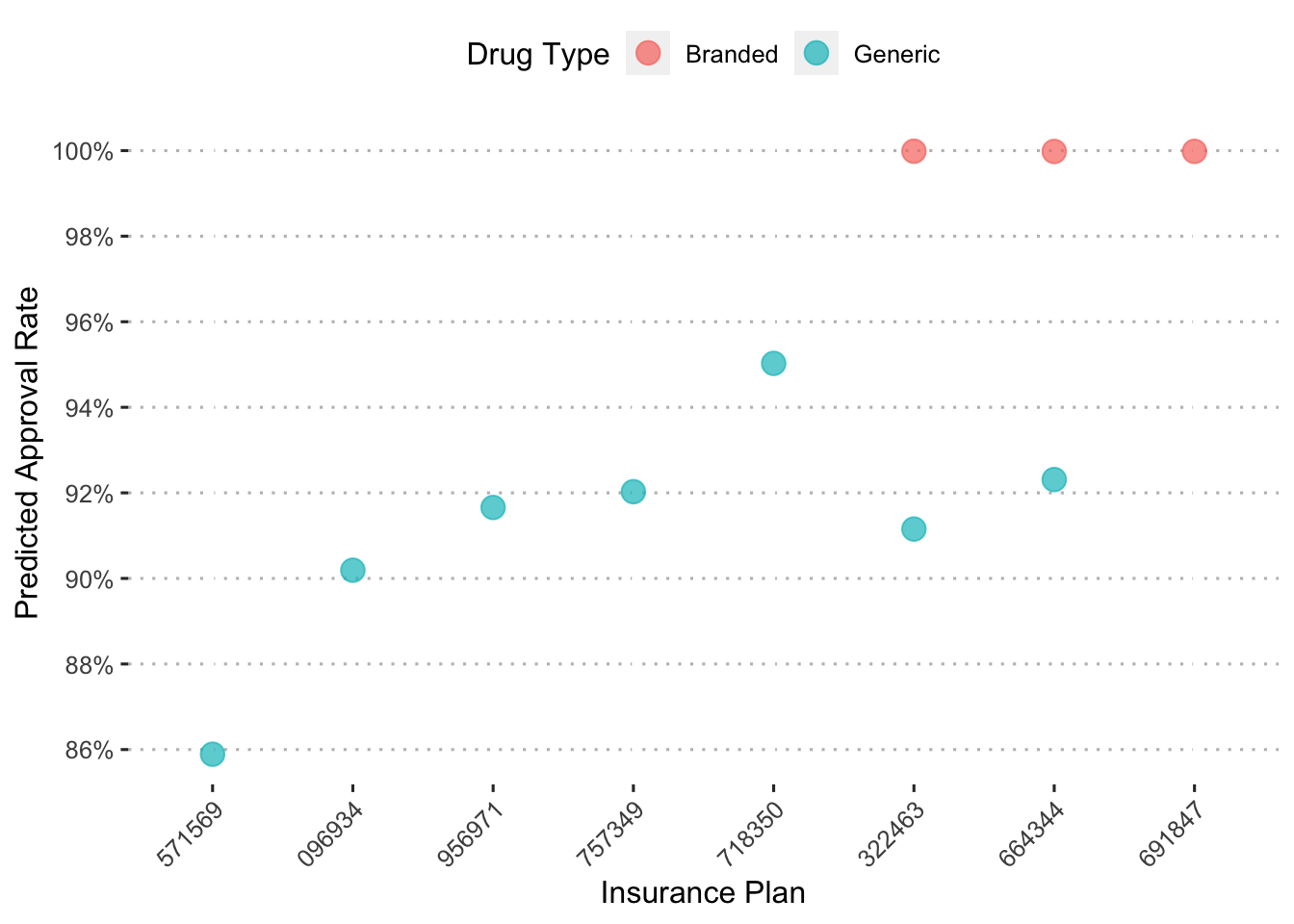

Constructing Formulary Status

To develop a measure of formulary status, I classify drugs into rejected, non-preferred, and preferred categories with the predicted probability of approval for each drug.

First, we’ll plot a histogram of the probabilities:

augment(final_c_fit) %>% 
  ggplot(aes(x = .pred_Approved)) +
  geom_histogram() +
  labs(x = "Predicted Approval Rate") +
  scale_x_continuous(breaks = pretty_breaks(n = 6), 
                     labels = percent_format()) +
  ggpubr::theme_pubclean()

## `stat_bin()` using `bins = 30`. Pick better value with `binwidth`.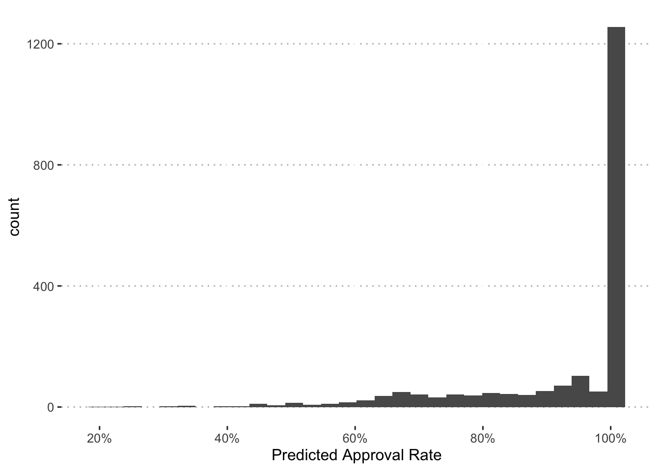

Based on this, we’ll use the following cutoffs:

90% - Preferred
< 90% & > 60% - Non-preferred
< 60% - Rejected

With these cut offs, we can examine the number of drugs that fall into each category.

augment(final_c_fit) %>% 
  group_by(bin, drug) %>% 
  summarize(pred_prob = mean(.pred_Approved)) %>% 
  mutate(f_status = case_when(
    pred_prob >= 0.90 ~ "Preferred",
    pred_prob < 0.90 & pred_prob >= 0.60 ~ "Non-Preferred",
    pred_prob < 0.60 ~ "Rejected"
  )) %>% 
  ggplot(aes(x = f_status)) +
  geom_bar() +
  labs(x = "Formulary Status", y = "Number of Drugs") +
  ggpubr::theme_pubclean()

## `summarise()` has grouped output by 'bin'. You can override using the `.groups`
## argument.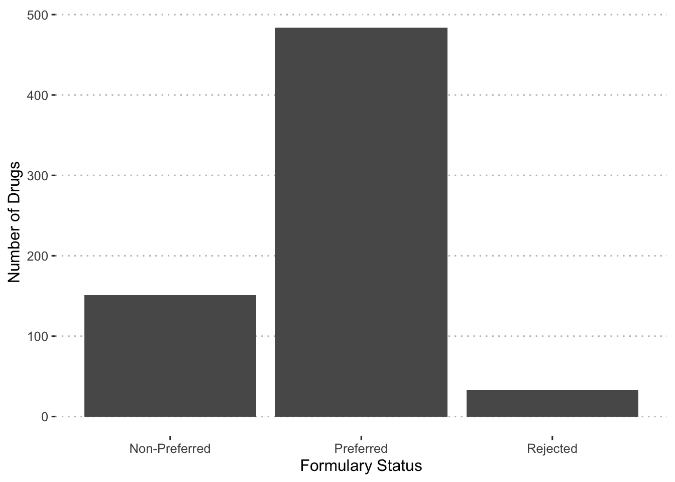

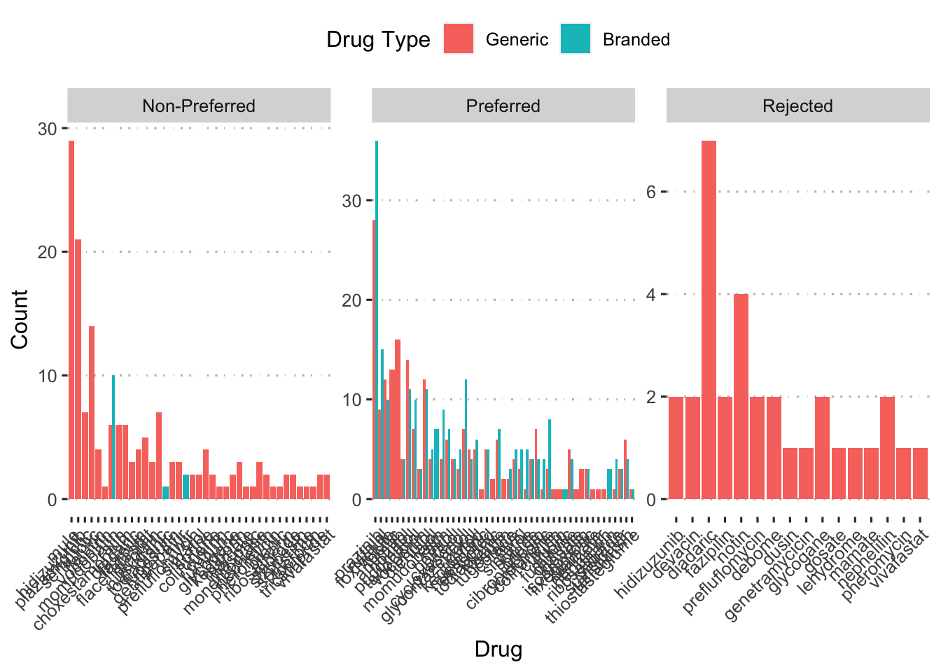
With a calculation of the formulary status, we can now examine which drugs fall into each group.

f_status_data <- 
  augment(final_c_fit) %>% 
  group_by(bin, drug) %>% 
  summarize(pred_prob = mean(.pred_Approved),
            n = n()) %>% 
  mutate(f_status = case_when(
    pred_prob >= 0.90 ~ "Preferred",
    pred_prob < 0.90 & pred_prob >= 0.60 ~ "Non-Preferred",
    pred_prob < 0.60 ~ "Rejected"
  ))

## `summarise()` has grouped output by 'bin'. You can override using the `.groups`
## argument.

f_status_data %>% 
  mutate(generic_drug = ifelse(str_detect(drug, "generic"), 1, 0),
         generic_drug = as_factor(generic_drug),
         drug_alt = str_replace(drug, "generic|branded", ""),
         drug_alt = str_trim(drug_alt, side = "both")) %>% 
  ggplot(aes(x = fct_reorder(drug_alt, n, .desc = TRUE), y = n, 
             fill = generic_drug)) +
  geom_col(position = position_dodge()) +
  facet_wrap(~ f_status, scales = "free") +
  labs(x = "Drug", y = "Count", fill = "Drug Type") +
  scale_fill_discrete(labels = c("Generic", "Branded")) +
  ggpubr::theme_pubclean() +
  theme(axis.text.x = element_text(angle = 45, hjust = 1))

Last updated on June 30, 2022