PACs and Small Dollar Donations: Data Visualization
Environment Preperation
This section clears the current working environment and loads the packages used to visualize the data. I also create the function comma() to format any in-line output values to have thousands separators and only two digits.
# Clear Environment -----------------------------------------------------------
rm(list = ls())

# Load Packages ---------------------------------------------------------------
library(pacman)
p_load(tidyverse, foreign, stargazer, maps, mapdata, maptools, ggmap,
       DataExplorer, ggpubr, ggthemes, scales)

# Inline Formatting -----------------------------------------------------------
comma <- function(x) format(x, digits = 2, big.mark = ",")

# Set Global Chunk Options ----------------------------------------------------
knitr::opts_chunk$set(
  echo = TRUE,
  warning = FALSE,
  message = FALSE,
  comment = "##",
  R.options = list(width = 70)
)
Import Data
This section imports the data cleaned in the “Step I: Data Cleaning” document to begin visualizing the data.
load("Data/Clean Data/estimation_data.RDa")

estimation.data <-
  estimation.data %>%
  mutate(chamber = str_sub(district, start = -2L, end = -1L),
         chamber = ifelse(str_detect(chamber, pattern = "S"), "Senate", "House"),
         vote_margin = vote_pct - 50) %>%
  filter(chamber == "House")
Data Visualization
plot_intro(estimation.data)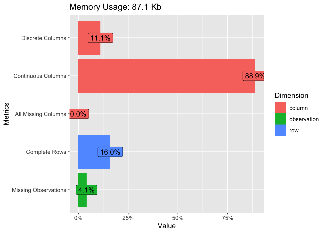
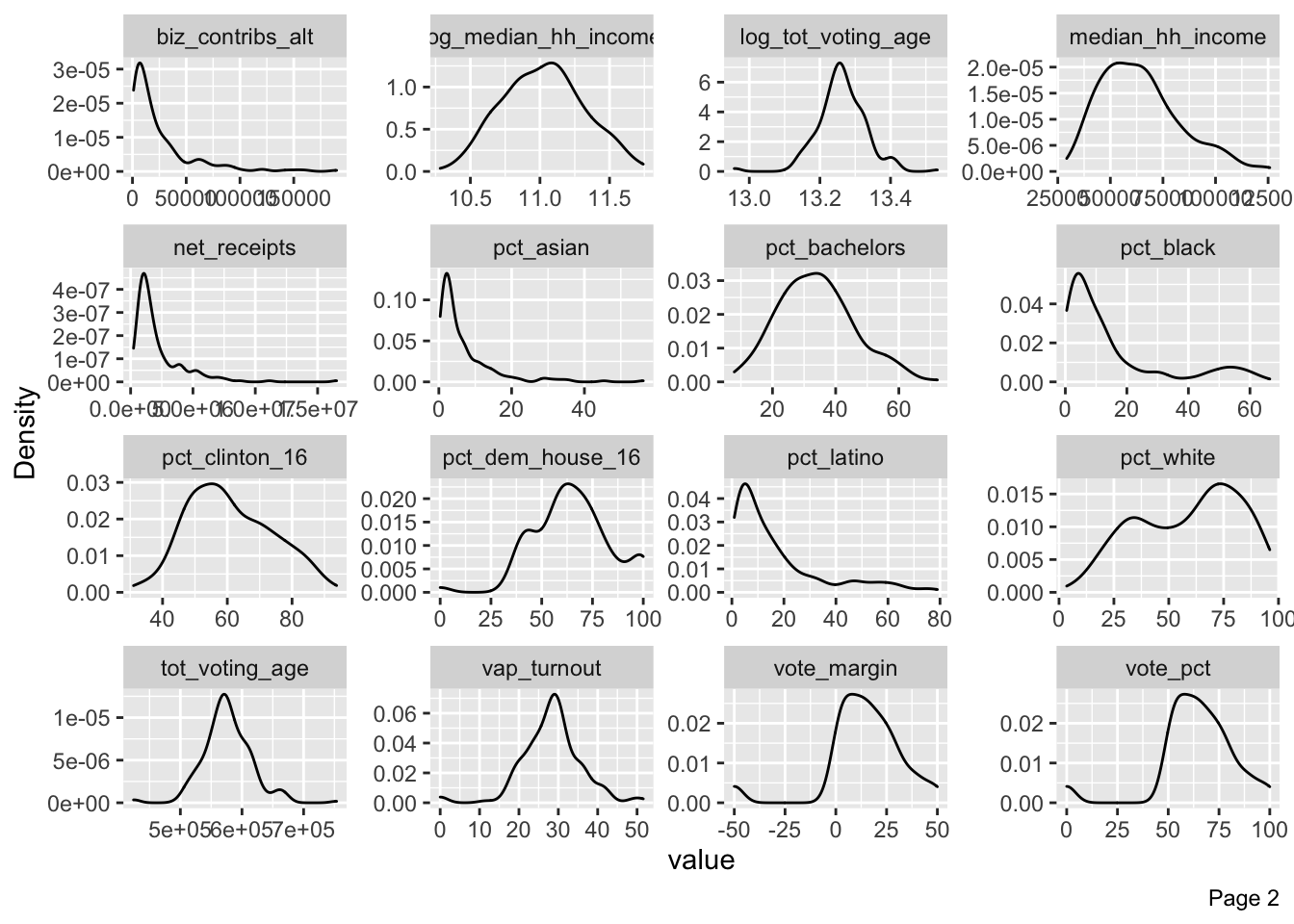
plot_density(estimation.data)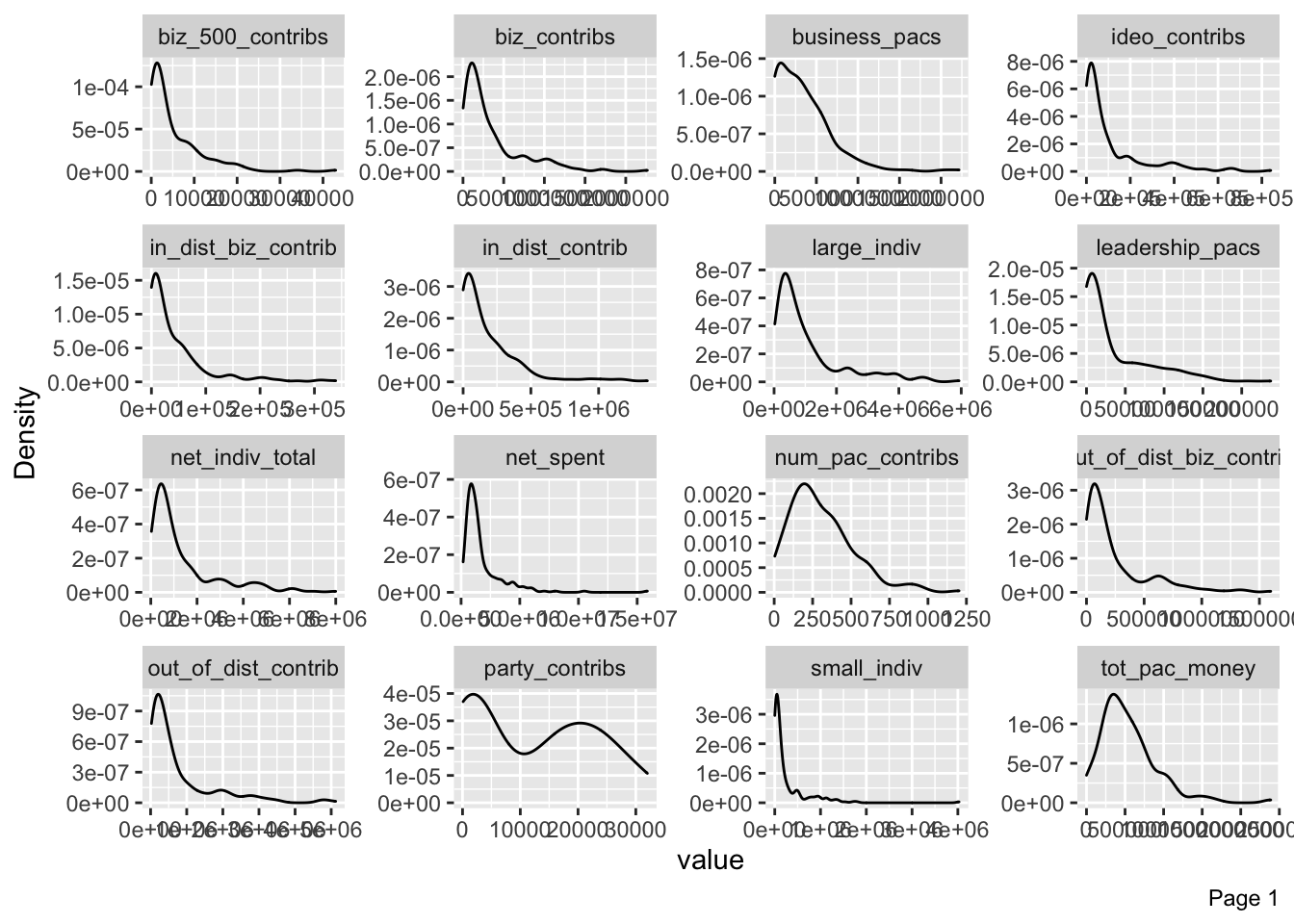
Plot Campaign Spending
plot.data <-
  estimation.data %>%
  select(no_corp_pacs, new_member, business_pacs, small_indiv, biz_contribs,
         out_of_dist_biz_contrib, net_spent, net_receipts) %>%
  pivot_longer(cols = c(business_pacs, small_indiv, biz_contribs,
                        out_of_dist_biz_contrib, net_spent, net_receipts),
               names_to = "group", values_to = "value") %>%
  mutate(group = factor(group,
                        levels = c("business_pacs", "small_indiv",
                                   "biz_contribs", "out_of_dist_biz_contrib",
                                   "net_spent", "net_receipts"),
                        labels = c("Business PAC $",
                                   "Small Indiv. $", "Business Indiv. $",
                                   "Out-of-District Business Indiv. $",
                                   "Net Spent", "Net Receipts"))) %>%
  group_by(group, no_corp_pacs) %>%
  summarise(sum = mean(value, na.rm = TRUE))

ggplot(data = plot.data %>%
         filter(group != "Net Spent" & group != "Net Receipts"),
       aes(x = fct_reorder2(group, no_corp_pacs, sum),
           y = sum,
           color = no_corp_pacs)) +
  geom_linerange(aes(x = fct_reorder2(group, no_corp_pacs, sum),
                     ymin = 0, ymax = sum),
                 color = "grey65",
                 size = 0.65,
                 position = position_dodge2(width = 0.7)) +
  geom_point(size = 6, position = position_dodge2(width = 0.7)) +
  #facet_wrap(~ fct_rev(no_corp_pacs)) +
  coord_flip() +
  scale_color_manual(values = c("grey71", "black"),
                     labels = c("No to Corporate PACs",
                                "Yes to Corporate PACs")) +
  labs(x = "", y = "Mean Contributions", color = "") +
  #guides(fill = FALSE, color = FALSE, linetype = FALSE, shape = FALSE)+
  scale_y_continuous(labels = dollar_format(), breaks = pretty_breaks(n = 8)) +
  theme_pubr()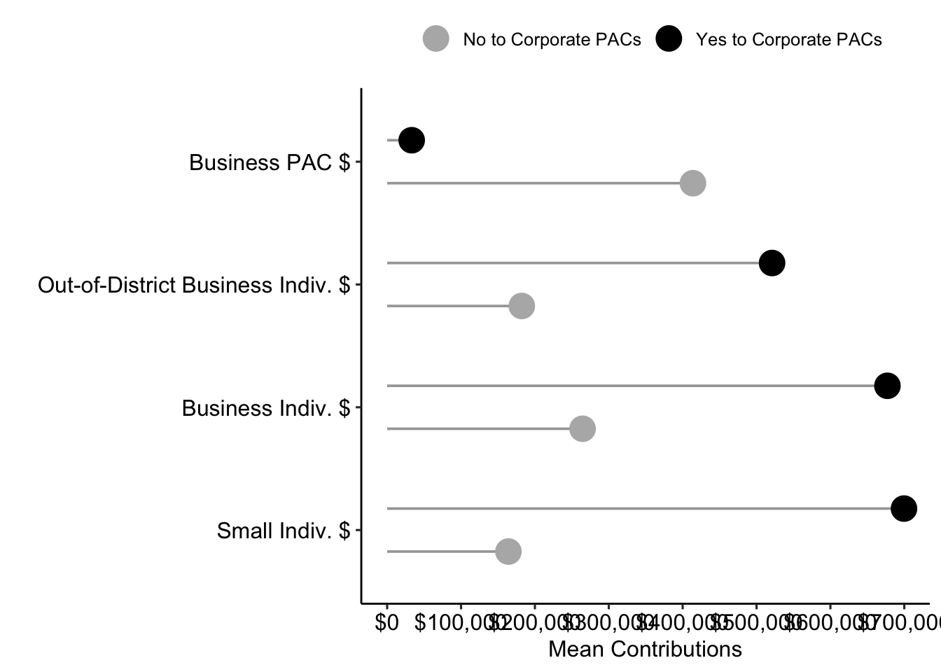
ggsave("Figures/all_candy.pdf", height = 4, width = 12)

# Spending and Receipts Plot
ggplot(data = plot.data %>%
         filter(group == "Net Spent" | group == "Net Receipts"),
       aes(x = fct_reorder2(group, no_corp_pacs, sum),
           y = sum,
           color = no_corp_pacs)) +
  geom_linerange(aes(x = fct_reorder2(group, no_corp_pacs, sum),
                     ymin = 0, ymax = sum),
                 color = "grey65",
                 size = 0.65,
                 position = position_dodge2(width = 0.5)) +
  geom_point(size = 6, position = position_dodge2(width = 0.5)) +
  #facet_wrap(~ fct_rev(no_corp_pacs)) +
  coord_flip() +
  scale_color_manual(values = c("grey71", "black"),
                     labels = c("No to Corporate PACs",
                                "Yes to Corporate PACs")) +
  labs(x = "", y = "Mean Contributions", color = "") +
  #guides(fill = FALSE, color = FALSE, linetype = FALSE, shape = FALSE)+
  scale_y_continuous(labels = dollar_format()) +
  theme_pubr()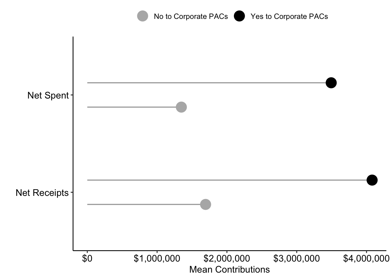
ggsave("Figures/spending_candy.pdf", height = 3, width = 12)

# Color Figures ---------------------------------------------------------------
plot.data <-
  estimation.data %>%
  select(no_corp_pacs, new_member, business_pacs, small_indiv, biz_contribs,
         out_of_dist_biz_contrib, net_spent, net_receipts) %>%
  pivot_longer(cols = c(business_pacs, small_indiv, biz_contribs,
                        out_of_dist_biz_contrib, net_spent, net_receipts),
               names_to = "group", values_to = "value") %>%
  mutate(group = factor(group,
                        levels = c("business_pacs", "small_indiv",
                                   "biz_contribs", "out_of_dist_biz_contrib",
                                   "net_spent", "net_receipts"),
                        labels = c("Business PAC $",
                                   "Small Indiv. $", "Business Indiv. $",
                                   "Out-of-District $",
                                   "Net Spent", "Net Receipts"))) %>%
  group_by(group, no_corp_pacs) %>%
  summarise(sum = mean(value, na.rm = TRUE))

ggplot(data = plot.data %>%
         filter(group != "Net Spent" & group != "Net Receipts") %>%
         mutate(group = factor(group,
                               levels = c("Small Indiv. $",
                                          "Business PAC $",
                                          "Business Indiv. $",
                                          "Out-of-District $")),
                sum_f = round(sum, 0)),
       aes(x = fct_rev(group),
           y = sum,
           color = no_corp_pacs,
           shape = no_corp_pacs,
           label = dollar(sum_f))) +
  geom_linerange(aes(x = group,
                     ymin = 0, ymax = sum),
                 color = "lightgray",
                 size = 2,
                 position = position_dodge2(width = 0.7)) +
  geom_point(size = 7, position = position_dodge2(width = 0.7)) +
  geom_label(position = position_dodge(width = 2.2),
             aes(x = group, y = sum, fill = no_corp_pacs),
             color = "white", fontface = "bold") +
  coord_flip() +
  scale_color_manual(values = c("#00AFBB", "#E7B800"),
                     labels = c("Yes to Corporate PACs",
                                "No to Corporate PACs")) +
  scale_fill_manual(values = c("#00AFBB", "#E7B800"),
                    labels = c("Yes to Corporate PACs",
                                "No to Corporate PACs")) +
  scale_shape_manual(values = c("NO" = 15, "YES" = 16),
                     labels = c("Yes to Corporate PACs",
                                "No to Corporate PACs")) +
  labs(x = "", y = "Average Amount of Money Received", color = "", shape = "") +
  guides(fill = FALSE, linetype = FALSE) +
  scale_y_continuous(labels = dollar_format(), breaks = pretty_breaks(n = 8)) +
  theme_pubclean(flip = TRUE)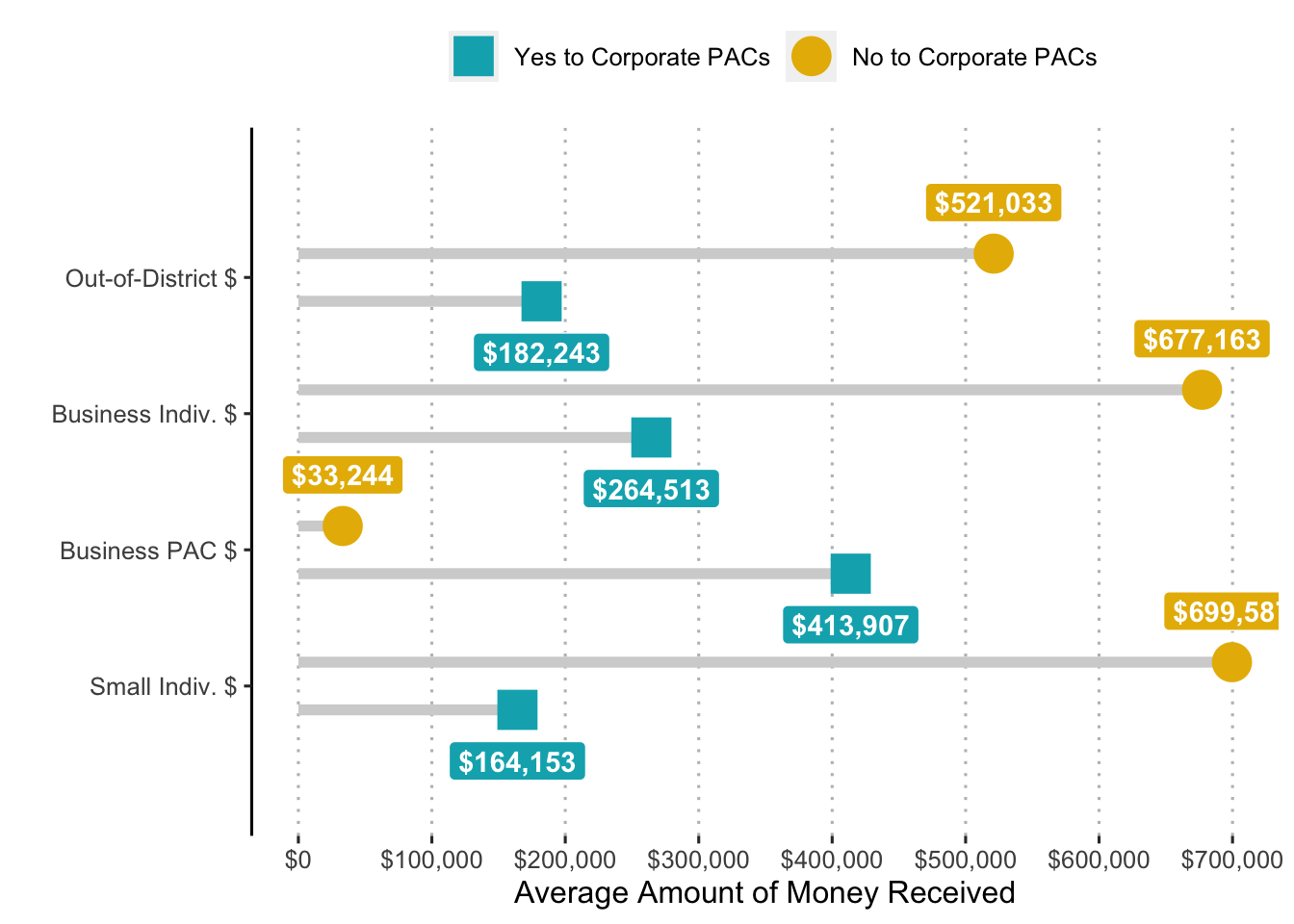
ggsave("Figures/all_candy_color_2.pdf", height = 5, width = 12)

# Spending and Receipts Plot
ggplot(data = plot.data %>%
         filter(group == "Net Spent" | group == "Net Receipts") %>%
         mutate(sum_f = round(sum, 0)),
       aes(x = fct_rev(group),
           y = sum,
           color = no_corp_pacs,
           shape = no_corp_pacs,
           label = dollar(sum_f))) +
  geom_linerange(aes(x = fct_reorder2(group, no_corp_pacs, sum),
                     ymin = 0, ymax = sum),
                 color = "lightgray",
                 size = 2,
                 position = position_dodge2(width = 0.7)) +
  geom_point(size = 6, position = position_dodge2(width = 0.7)) +
  geom_label(position = position_dodge(width = 2.2),
             aes(x = group, y = sum, fill = no_corp_pacs),
             color = "white", fontface = "bold") +
  coord_flip() +
  scale_color_manual(values = c("#00AFBB", "#E7B800"),
                     labels = c("Yes to Corporate PACs",
                                "No to Corporate PACs")) +
  scale_fill_manual(values = c("#00AFBB", "#E7B800"),
                    labels = c("Yes to Corporate PACs",
                                "No to Corporate PACs")) +
  scale_shape_manual(values = c("NO" = 15, "YES" = 16),
                     labels = c("Yes to Corporate PACs",
                                "No to Corporate PACs")) +
  labs(x = "", y = "Mean Contributions", color = "", shape = "") +
  guides(fill = FALSE, linetype = FALSE) +
  scale_y_continuous(labels = dollar_format(), breaks = pretty_breaks(n = 8)) +
  theme_pubclean(flip = TRUE)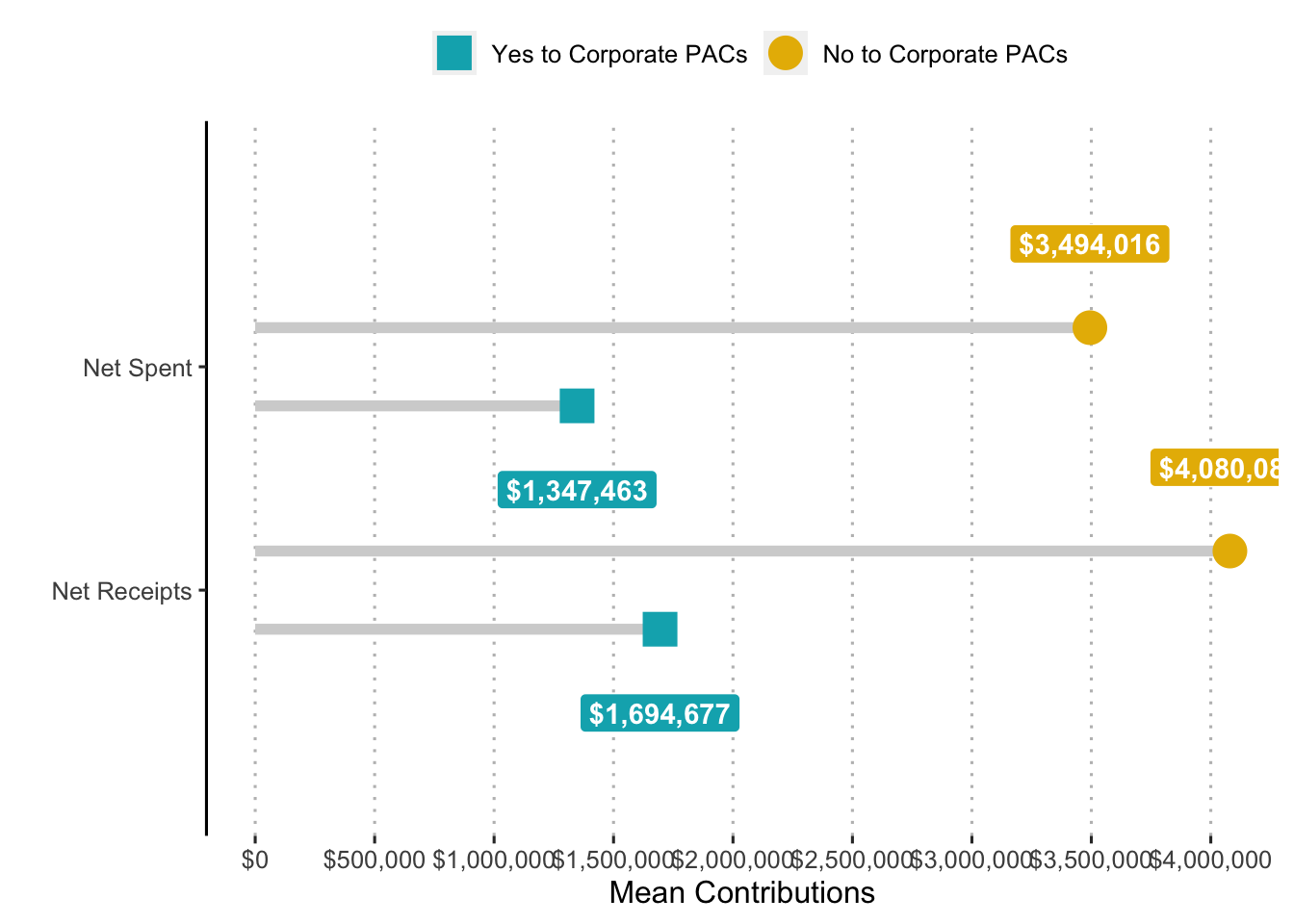
ggsave("Figures/spending_candy_color.pdf", height = 3, width = 12)Other Descriptives
summary(estimation.data$no_corp_pacs)## NO YES
## 193 44Plot Zeros
zeros <-
  estimation.data %>%
  select(business_pacs, small_indiv, biz_contribs, out_of_dist_biz_contrib) %>%
  mutate(out_of_dist_biz_contrib = ifelse(is.na(out_of_dist_biz_contrib), 0,
                                          out_of_dist_biz_contrib)) %>%
  summarise(business_pacs = sum(business_pacs == 0),
            small_indiv = sum(small_indiv == 0),
            biz_contribs = sum(biz_contribs == 0),
            out_of_dist_biz_contrib = sum(out_of_dist_biz_contrib == 0)) %>%
  mutate_at(vars(business_pacs:out_of_dist_biz_contrib), ~ . / nrow(estimation.data)) %>%
  pivot_longer(cols = c(business_pacs, small_indiv, biz_contribs,
                        out_of_dist_biz_contrib),
               names_to = "model", values_to = "zeros")

ggdotchart(data = zeros,
           x = "model",
           y = "zeros",
           sorting = "descending",
           add = "segments",
           rotate = TRUE,
           dot.size = 6,
           label = round((zeros$zeros) * 100),
           font.label = list(color = "white", size = 9,
                             vjust = 0.5),
           color = "black",
           ggtheme = theme_pubr()) +
  scale_y_continuous(labels = percent_format()) +
  scale_x_discrete(labels = c("Small Indiv. $", "Business Indiv. $",
                              "Business PAC $",
                              "Out-of-District Business Indv. $")) +
  labs(y = "Percantage of Zeros", x = "")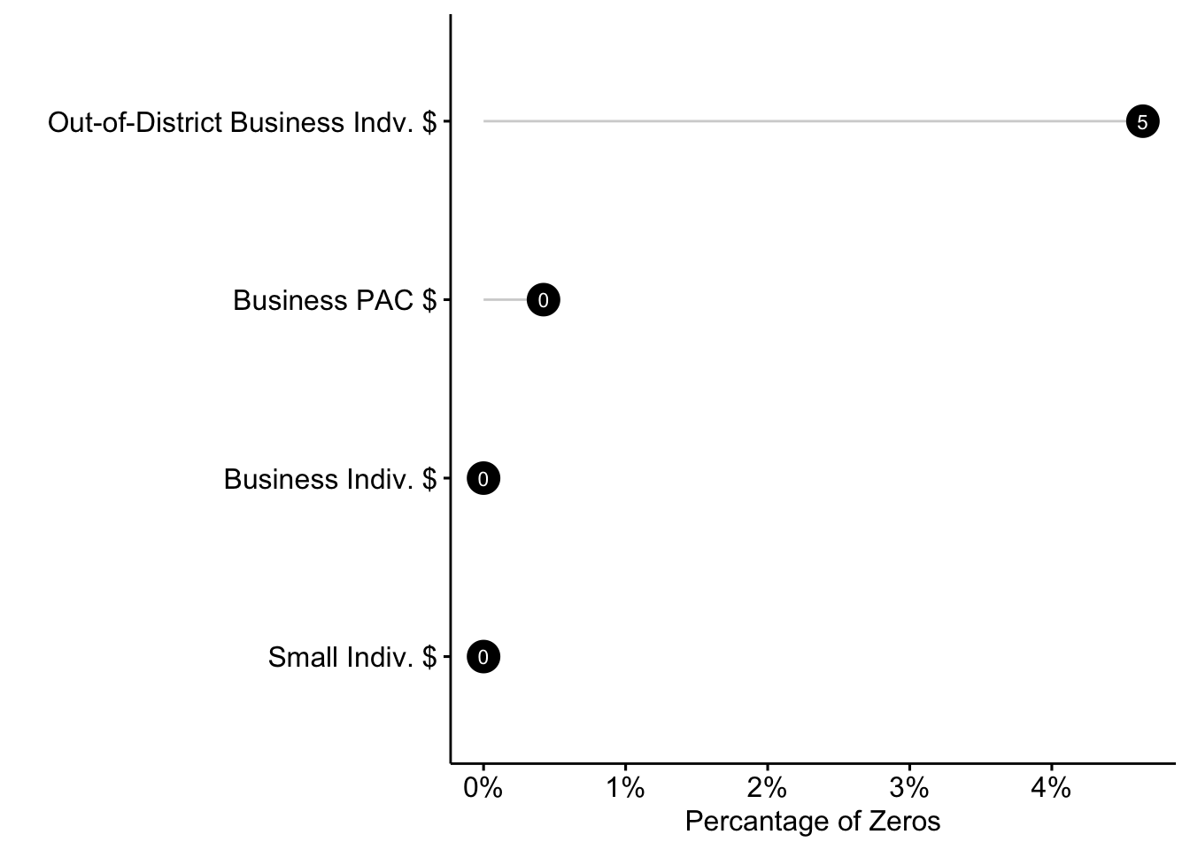
ggsave("Figures/zero_candy.pdf", height = 3, width = 8)Nominate Scores
nominate.data <- read_csv("Data/Raw Data/HSall_members.csv")

nominate.data <-
  nominate.data %>%
  filter(congress == 116) %>%
  filter(party_code == 100) %>%
  select(state_abbrev, district_code, nominate_dim1, nominate_dim2, party_code) %>%
  mutate(district_code = str_pad(district_code, pad = 0, side = "left",
                                 width = 2),
         district = str_c(state_abbrev, district_code, sep = "")) %>%
  filter(str_detect(district, "00", negate = TRUE))

nominate.data %>%
  group_by(district) %>%
  summarise(n = n()) %>%
  arrange(desc(n))
## # A tibble: 235 × 2
## district n
## <chr> <int>
## 1 GA05 2
## 2 MD07 2
## 3 AL07 1
## 4 AZ01 1
## 5 AZ02 1
## 6 AZ03 1
## 7 AZ07 1
## 8 AZ09 1
## 9 CA02 1
## 10 CA03 1
## # … with 225 more rowsestimation.data <-
left_join(estimation.data,
nominate.data,
by = "district")
estimation.data %>%
group_by(party_code) %>%
summarise(d1_min = min(nominate_dim1, na.rm = T),
d1_max = max(nominate_dim1, na.rm = T),
d2_min = min(nominate_dim2, na.rm = T),
d2_max = max(nominate_dim2, na.rm = T))## # A tibble: 2 × 5
## party_code d1_min d1_max d2_min d2_max
## <dbl> <dbl> <dbl> <dbl> <dbl>
## 1 100 -0.725 -0.069 -0.975 0.84
## 2 NA Inf -Inf Inf -Infestimation.data %>%
group_by(no_corp_pacs) %>%
summarise(dim1_mean = mean(nominate_dim1, na.rm = T),
dim2_mean = mean(nominate_dim2, na.rm = T))## # A tibble: 2 × 3
## no_corp_pacs dim1_mean dim2_mean
## <fct> <dbl> <dbl>
## 1 NO -0.383 -0.0156
## 2 YES -0.312 0.0978estimation.data %>%
mutate(`Candidate Accepts Corporate PAC Money?` = factor(no_corp_pacs,
levels = c("NO", "YES"),
labels = c("Yes", "No"))) %>%
ggplot(aes(x = nominate_dim1, y = nominate_dim2,
shape = `Candidate Accepts Corporate PAC Money?`,
color = `Candidate Accepts Corporate PAC Money?`)) +
geom_point(size = 2, fill = "black") +
annotate("text", x = 0.35, y = -0.6, label = "D1 Means", fontface = 2) +
annotate("text", x = 0.35, y = -0.72, label = "Acceptors: -0.38") +
annotate("text", x = 0.35, y = -0.82, label = "Rejectors: -0.30") +
annotate("text", x = -0.90, y = 0.95, label = "D2 Means", fontface = 2) +
annotate("text", x = -0.90, y = 0.85, label = "Acceptors: -0.02") +
annotate("text", x = -0.90, y = 0.75, label = "Rejectors: 0.11") +
labs(x = "DW-Nominate Dimension 1: Economic/Redistributive Issues",
y = "DW-Nominate Dimension 2: Social/Lifestyle Issues") +
scale_x_continuous(limits = c(-1, 0.5)) +
scale_y_continuous(limits = c(-1, 1)) +
scale_color_manual(values = c("grey71", "black")) +
scale_shape_manual(values = c(20, 24)) +
theme_pubr()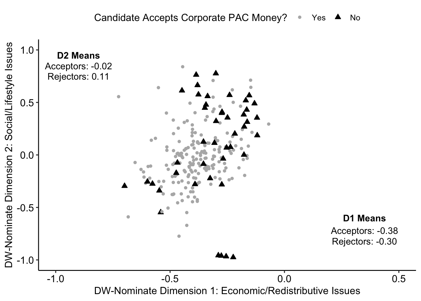
ggsave("Figures/nominate_plot.pdf", plot = last_plot(), width = 7, height = 5)

estimation.data %>%
  mutate(`Candidate Accepts Corporate PAC Money?` = factor(no_corp_pacs,
                                                           levels = c("NO", "YES"),
                                                           labels = c("Yes", "No"))) %>%
  ggplot(aes(x = nominate_dim1, y = nominate_dim2,
             shape = `Candidate Accepts Corporate PAC Money?`,
             color = `Candidate Accepts Corporate PAC Money?`,
             fill = `Candidate Accepts Corporate PAC Money?`)) +
  geom_point(size = 5, alpha = 0.7,
             position = position_jitterdodge(jitter.width = 0.2, dodge.width = 0.2)) +
  geom_hline(yintercept = 0, linetype = 2) +
  geom_vline(xintercept = 0, linetype = 2) +
  annotate("text", x = 0.35, y = -0.65, label = "Mean Economic Scores", fontface = 2) +
  annotate("text", x = 0.35, y = -0.77, label = "Acceptors: -0.38") +
  annotate("text", x = 0.35, y = -0.87, label = "Rejectors: -0.30") +
  annotate("text", x = -0.85, y = 0.90, label = "Mean Social Scores", fontface = 2) +
  annotate("text", x = -0.85, y = 0.80, label = "Acceptors: -0.02") +
  annotate("text", x = -0.85, y = 0.70, label = "Rejectors: 0.11") +
  labs(x = "Economically Liberal                                  Economically Conservative",
       y = "Socially Liberal        Socially Conservative",
       caption = "Data points are 1st and 2nd Dimention DW-NOMINATE scores.") +
  scale_x_continuous(limits = c(-1, 0.5)) +
  scale_y_continuous(limits = c(-1, 1)) +
  scale_color_manual(values = c("#00AFBB", "#E7B800"),
                     labels = c("Yes", "No")) +
  scale_fill_manual(values = c("#00AFBB", "#E7B800"),
                    labels = c("Yes", "No")) +
  scale_shape_manual(values = c(21, 24),
                     labels = c("Yes", "No")) +
  theme_pubr() +
  theme(axis.line.x = element_line(arrow = grid::arrow(length = unit(0.5, "cm"),
                                                       ends = "both",
                                                       type = "closed")),
        axis.title.x = element_text(angle = 0),
        axis.line.y = element_line(arrow = grid::arrow(length = unit(0.5, "cm"),
                                                       ends = "both",
                                                       type = "closed")),
        axis.title.y = element_text(angle = 90),
        axis.text = element_blank(),
        axis.ticks = element_blank())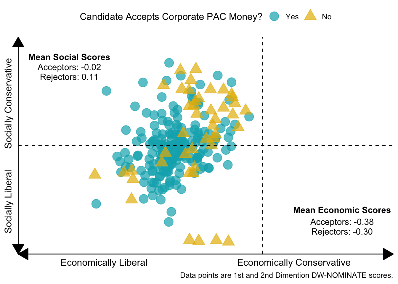
ggsave("Figures/nominate_plot_color.pdf",
       plot = last_plot(), width = 7, height = 5)